
Archimedes uses resonant mass measurement (RMM) to measure the buoyant mass of particles suspended in fluid. This is the effective mass of the particle in the fluid, as the upward force of buoyancy will offset, or overcome, the downward force of the particle’s weight. According to the Archimedes principle, buoyant mass is equal to the mass of the fluid displaced by the particle subtracted from the mass of the particle, as seen in Equation 1.
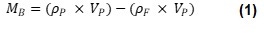
Where ρP is particle density, VP is particle volume, ρF is fluid density and MB is buoyant mass. Equation 1 can be simplified to Equation 2:
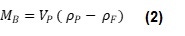
Equation 2 shows that when a particle has the same density as the fluid in which it is submerged, it will have a buoyant mass of zero, when ρP = ρF, MB = 0. This relationship can be used to measure the density of a particle when its size is unknown. If the buoyant mass of the same particle is measured in at least two fluids of different densities, these values can be plotted on a graph of buoyant mass vs. fluid density. The resulting points can then be used to plot a line and find the y-intercept, giving the fluid density at which MB = 0, hence the particle density, as shown in Figure 1.
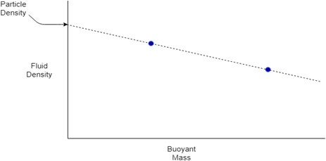
Figure 1. A sketch graph demonstrating how particle density can be measured
As with all measurements, the calibration of the Archimedes should be checked, ensuring that it is in-line with specifications. It is recommended that at least three repeat measurements are performed in each fluid and that at least 500 particles are measured per replicate. These settings may vary depending on the nature and availability of the sample.
It is also advised that the different fluids used in these measurements have a significant difference in density in comparison to the estimated density of the material being measured. Furthermore, while an extrapolation can be performed with only 2 points, it is strongly suggested that at least 3 different fluids are used to improve the accuracy of the method.
The ideal fluids used for these measurements will depend on the sample that is being measured and its stability in different dispersants. For example, if the sample is stable in water it can also be measured in D2O, or D2O/H2O mixtures to achieve different fluid densities. Sucrose solutions can also be used as an alternative to D2O. If stable in organic solvents, ethanol can be used for a much lower fluid density.
If the density of the carrier fluid is unknown, it can be calculated using the fluid density calculator in the Archimedes software, as shown in Figure 2. This is done by measuring a fluid of a known density (calibration fluid) and recording its resonant frequency from the experiment info window on the left side of the screen. This can then be entered into the fluid density calculator, along with the resonant frequency of the sample fluid to calculate the sample fluid density, as shown in Figure 3.
Figure 2. Archimedes Software Toolbar. Density calculator highlighted by red circle
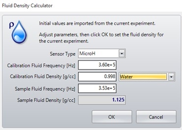
Figure 3. Fluid density calculator window - can be used when the density of the fluid being used is unknown
When measuring the sample of interest, you will be prompted to enter a density for the particle you are measuring. A rough estimate can be used, as this value is only used in the calculation of particle size and not in the measurement of buoyant mass, as shown in Figure 4.
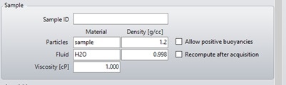
Figure 4. The particle acquisition window - an estimate for particle density can be used at this stage
To calculate particle density, the modal buoyant mass in each fluid is required. To obtain this in the Archimedes software, right-click the x-axis of the histogram in the Archimedes software and select 'buoyant mass', as shown in Figure 5.
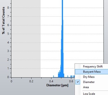
Figure 5. Screenshot of the dropdown menu allowing the x-axis of the histogram in the Archimedes software to be changed
Following this, the modal buoyant mass can be obtained from the particle statistics window to the right of the graph, as shown in Figure 6.
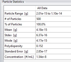
Figure 6. Particle statistics window, showing the modal buoyant mass of the sample.
These data are then used to calculate an average value for modal buoyant mass in each fluid and a buoyant mass vs. fluid density graph can be plotted in a third-party analysis tool such as Microsoft Excel or Minitab, and the y-intercept extrapolated or read from the graph.
If using Microsoft Excel, first plot a scatter graph using the measured data. Next, add a trendline and tick the 'Display Equation on chart' box under 'Format Trendline'. This will give you the y-intercept of the plotted trendline and hence the particle density.
The determined particle density can be used to recalculate the particle mass and size by inputting the new value into the experiment info window, as shown in Figure 7.
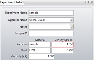
Figure 7. The experiment info window. The particle density can be changed here to recalculate particle size after the measurement is finished.
Below is a set of results from measuring a sample of NIST certified 1µm latex nanospheres. The specification lists the density of these particles as 1.05 gcm-3.
Four H2O/D2O mixtures were prepared at 0%, 25%, 75% and 100% D2O. The sample was diluted to the necessary concentration at approximately 9.0x10⁶ particles/ml. Three repeat measurements were made for each fluid, with the fluid density being measured simultaneously through Archimedes density calculator. An average modal buoyant mass was calculated for each fluid density.
As expected, the buoyant mass for latex transitions from a positive value to a negative value when it is measured in fluids that are more dense than itself, Table 1).
| %D2O | Fluid Density / gcm-3 | Buoyant Mass / 10-14 g |
| 0 | 0.997 | 2.34 |
| 25 | 1.021 | 1.29 |
| 75 | 1.077 | -1.37 |
| 100 | 1.104 | -2.63 |
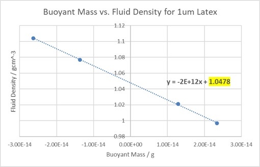
Figure 8. A graph showing the change in the buoyant mass of latex when measured in different fluid densities.
The displayed equation shows that the y-intercept (highlighted) is at approximately 1.048 gcm-3, very close to the specification value of 1.05gcm-3. Repeating these measurements twice more gave a mean density of 1.0481 ± 0.001 gcm-3, showing the high precision of the method when measuring this sample.
This method is very applicable for lower density particles, giving accurate and precise density values even when the particle size is unknown. However, the method becomes less effective as the density of the particles being measured is increased. Looking at Equation 2, it can be seen that when ρP is much greater than ρF, the ρP - ρF term will approach the constant value of ρP. Hence, MB will stay effectively constant regardless of ρF, preventing any meaningful extrapolation. To offset this effect, fluids with greater densities will be required for measuring higher density particles. However, this becomes less feasible at very high densities, such as metal particles, where this method would not be suitable.
Another factor to consider is the polydispersity of the sample. Equation 2 shows that buoyant mass is affected by particle density, fluid density and particle volume. Particle density will be a constant, however particle volume is dependent on the size of the particle. The size of the particles measured for each point on the graph need to be the same to achieve accurate data. This is why it is recommended to plot the modal buoyant mass rather than the mean, as the mode represents a much smaller range of particle sizes than the mean when measuring samples with a wide size distribution. Should a sample contain multiple size populations, the modal buoyant mass for each can be obtained separately by adjusting the cursors (shown by right clicking the graph and selecting the ‘cursors’ option) on the histogram in the Archimedes software to only include data from the population of interest, Figure 9.
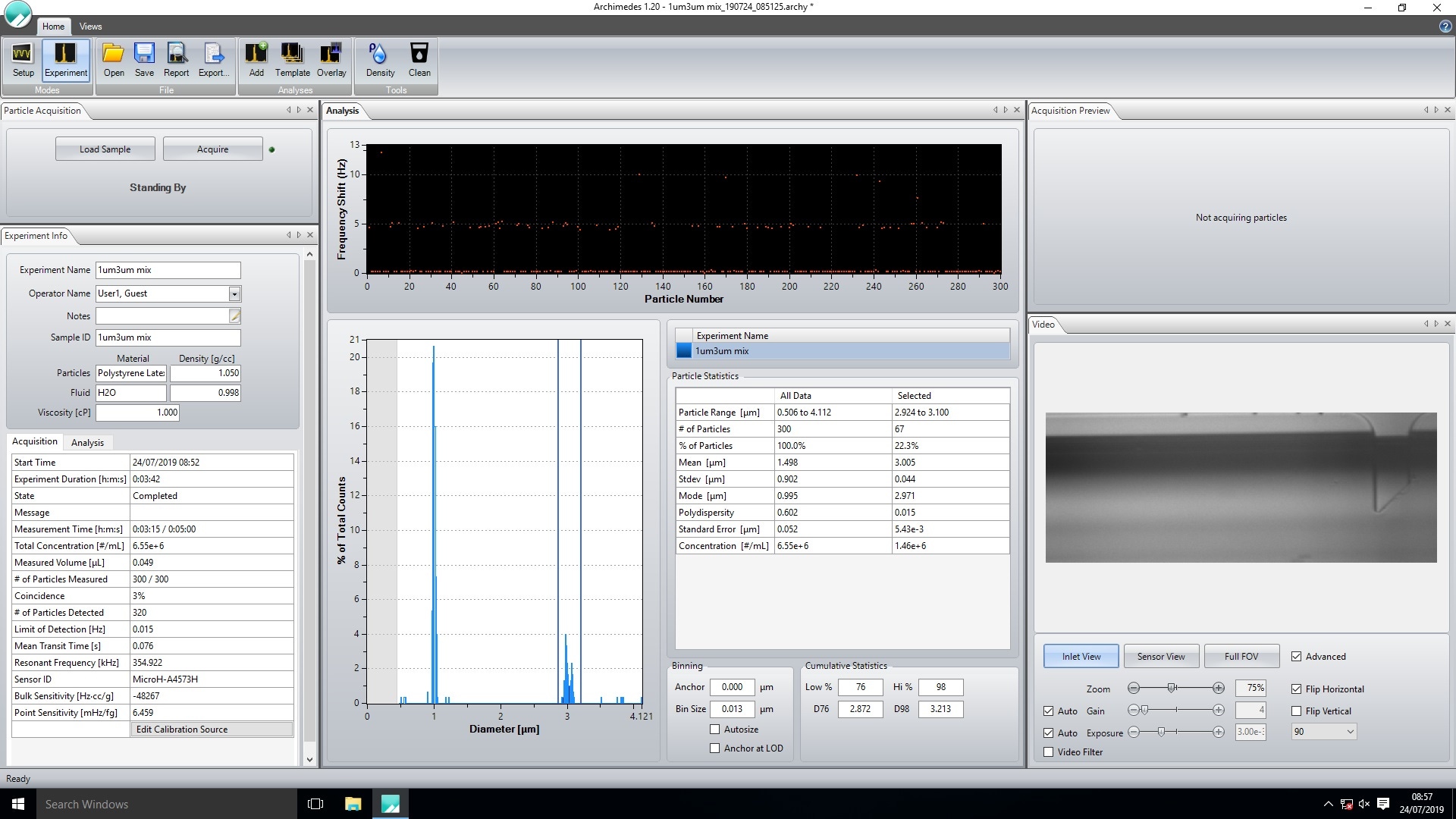
Figure 9. Using the cursors in the Archimedes software to select a population of interest.