The measurement of zeta potential is performed by first measuring a quantity known as electrophoretic mobility then converting that value by applying electrokinetic theory to zeta potential. Mobility is defined as the velocity of a particle in a unit electrical field. In practice as high an electric field is applied as is possible or desirable: the field and velocity are measured as accurately as possible and the electrophoretic mobility is derived from the simple relationship:
Mobility = Velocity/Electric field
Zeta potential, and hence mobility, can be either positive or negative in sign, and hence the direction of travel depends on the sense of the electric field.
The electronics fitted to the Nano are able to make accurate measurements of the applied field under all measurement conditions so the final accuracy of the result depends on the ability to the measure particle velocity.
Velocity is measured by detecting the change in frequency of light scattered by the particles, the well known 'Doppler Effect'. In the Zetasizer Nano, the method of Phase Analysis Light Scattering is utilized. This measures the frequency change by comparing the relative phase of the scattered signal with that of a reference signal, and is very sensitive so that small frequency shifts can be measured. In the Zetasizer Nano, this reference is generated by an optical modulator at a frequency of between 250 and 320 Hertz. This enables signals above and below the modulator to be recognized and the electric field is applied so that higher frequencies correspond to positively charged particles and lower to negative.
By definition …phase = frequency x time, so measuring the change in phase as a function of time enables the frequency shift and hence mobility to be determined. The field is reversed periodically with a period of between 26 and 45 milliseconds. These periods are set for different measurement conditions in different designs of cell.
Since frequency shift is proportional to mobility x electric field, it would seem that in order to determine a small value of mobility, one could simply increase the field to higher values. In practice, there are limitations due to the conductivity of many types of sample. The possibility of electrical breakdown even in non-conductive samples limits the electric fields that can be used safely. It is better to use the ability of PALS to make accurate measurements of small frequency changes than to increase the applied field.
In order to make a measurement, several reversals of the electric field are applied successively in a burst known as a 'run'. The field reversal is to ensure the net field in each direction is the same and to reduce any polarization effects such as the evolution of gas at the electrodes.
One run is almost never sufficient as the particles are in random motion, (Brownian motion) and these movements need to be averaged out. There are also systematic fluid flows due to convection and the additional (Joule) heating effect of passing an electric current through a conductive medium. The result of all these other effects is to add random phase changes to the systematic changes caused by the electrophoretic mobility of the sample. The mobility effects are synchronized with the changes in the direction of the applied field, while the thermal and other random motion effects are not. It is possible to add runs together so that the noise effects tend to cancel while the systematic electrophoretic effects reinforce.
The matter then is to decide how many runs to perform to get an acceptable result, and to know how accurate the result is based on calculations on the data itself. The measurement can then also be repeated on the same sample, and also different aliquots of the sample, to see that consistent results are obtained.
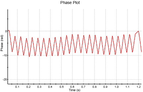
The phase plot of a measurement of a transfer standard test material material is shown below. This is considered an 'easy' sample as its mobility is relatively high. (Typical electrophoretic mobility values range from -10 to + 10 expressed in these obsolete but convenient units)
It can be seen from the figure the regular saw-tooth waveform created by the field switching, superimposed on a wavy background caused by the thermal drifts also present. In this case the signal - the saw tooth - is much larger than any higher frequency noise and easily distinguished from the slower background drift.
|
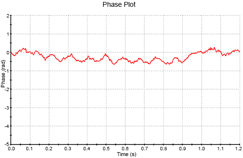
In figure 2 we see that the noise appears to be larger than any systematic electrophoretic signal. The data could probably be improved by running a longer measurement, but what is needed is some objective way of measuring the ratio of signal to noise in a phase plot so as to 'know' how long to continue measuring and then to assess how accurate the result is.
|
In version 5.00 software and later versions, we have integrated the calculation of a quality factor designed to perform this function. Since the signal has a fundamental component at the frequency of the applied field while the noise is expected to be present at all frequencies, we compare the power in the phase spectrum at the field frequency with the average power at other frequencies. This is done internally by performing a Fourier Transform on the data and picking out the peak at the expected frequency arising from the electrophoretic effect.
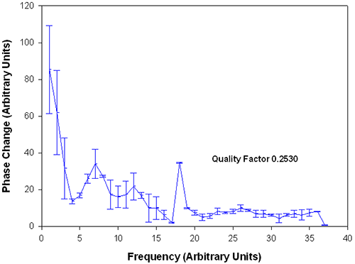
Figure 3 shows an example of a more 'difficult' sample in that it is a low mobility material. The mobility value of -0.1 makes it some 40 times more 'difficult' than the test material used before. After 1 run we can just pick out a peak at channel 18 which corresponds to applied field frequency. The area under this peak is compared to the noise level (represented by the error bars on the frequency data adjacent to the peak) and the ratio calculated and scaled in such a way the 'good' data will have a value > 1. The noise is estimated by variations in the spectrum from channel to channel. In this case, the channels used to estimate the noise go from 10 to 16 and 20 to 35: the peak from 17 to 19. (This selection depends on the actual frequency of the field which can have different settings).
|
Note that at low frequencies the noise error bars are around +/- 20 units, at higher frequencies +/- 5 or less compared to a peak height of 40. A quality factor of 0.25 was computed for this single run so a longer measurement is needed (figure 3).
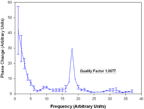
Figure 4 shows that after 150 runs, the quality factor has increased to 1.07 (figure 4). The peak now reaches 30 units from a lower baseline while the noise levels as represented by the error bars on the spectrum are now of the order +/- 1.5 below the peak and less than that at higher frequencies.
|
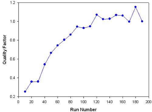
Figure 5 demonstrates graphically how the quality factor varied during this measurement. In this case the quality factor is plotted every 10 runs.
|
Note that after about 120 runs the quality tends to level off and more runs will not produce a marked improvement. This effect is to be expected as the measurement is not simply limited by random noise. The measurement process itself induces further noise due to the passage of electric current and possible degradation of sample and electrodes. Further improvement might well involve much longer run times. In this case, as the target value of 1 is reached after about 120 runs, the automatic measurement duration will stop, providing the result remains stable.
For very low mobility samples, it is necessary to perform a minimum number of measurements before the quality factor can be relied on. This is because random fluctuation in the phase spectrum will take place in the 'peak' as well as the regions to either side so spuriously 'good' values can be obtained from a few runs.
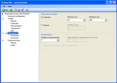
The automatic measurement is normally set up so that there is a minimum of 10 runs and a maximum of 100 (Figure 6). The measurement will therefore stop sometime after 10 but before 100 runs if the quality factor of 1 has been attained. These run number settings are alterable by the user. Shortening the automatic duration below the level set is not recommended. It is of course possible to perform a manual measurement of any number of runs. The quality factor can be displayed in the record view or on another report as required. It is used by the 'expert system' to determine if sufficient runs have been performed.
|
Having performed a measurement that obtains a good quality factor, how good is that measurement? To calculate the mobility, the phase change as a function of time - ie the gradient of the saw tooth segments in the phase plot is calculated. To do this, the separate field reversals throughout the run data are averaged and a linear fit performed. In addition to calculating the gradient, the relative error in the gradient and also the correlation coefficient R that determines if the phase data actually are well represented by a straight line, are calculated.
In table 1, it can be seen that from a data fitting point of view, a good quality result will likely have a mobility error of 0.01, i.e. +/- 1% of the mobility value. This seems to be a good target to achieve. It is then recommended that measurements are made on several samples, and the run variation determined, which is likely to be larger than the uncertainty from the data analysis.
| Quality Factor | Relative Mobility Error | Correlation Coefficient |
|---|---|---|
| 2 to 5 | 0.01 | 0.999 |
| 1.0 | 0.015 | 0.995 |
| 0.5 | 0.02 | 0.992 |
| 0.25 | 0.08 | 0.957 |