The Zetasizer ZS Xplorer software is a powerful tool for size and zeta potential measurements. There are several ways for you to customize your workspace and tables in the software with an abundance of parameters to choose from. Understanding the meaning behind all the terms enables you to appreciate both the hardware and software’s versatility. Furthermore, having a glossary of these terms provides valuable insight.
The Zetasizer ZS Xplorer software is a powerful tool for size and zeta potential measurements. There are several ways for you to customize your workspace and tables in the software with an abundance of parameters to choose from. Understanding the meaning behind all the terms enables you to appreciate both the hardware and software’s versatility. Furthermore, having a glossary of these terms provides valuable insight.
One of the ways to access the different terms, is to select Analyze Tab in the menu bar:

Then select the “Customs” Tab and create a “Parameter Table” in the workspace:
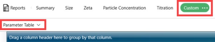
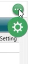
Once you create the parameter table, you can view the full list of parameters by clicking on the three dots in the upper right corner and clicking the cog:
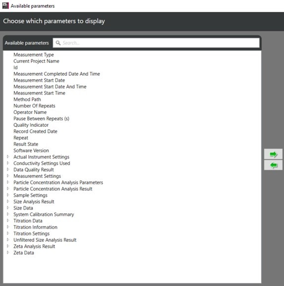
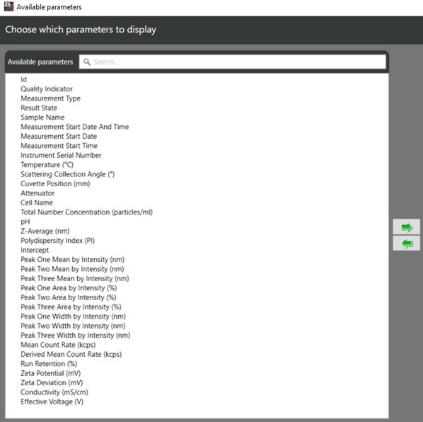
Once you see the separate Parameters window, expand all the options, and see the full list of terms:
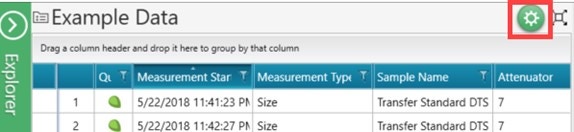
Alternatively, you can access a shorter list of parameters by clicking on the cog in the upper right corner of the Record Selector:
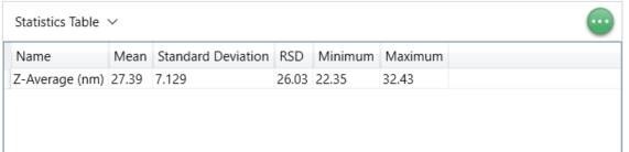
Furthermore, you can also access a short list of parameters by creating a Statistics Table:
Please find the list of definitions for each parameter from both windows below.
Parameter | Definition | |||
|---|---|---|---|---|
| Number of Repeats | Number of repeat measurements within a group of a selected measurement type. | |||
| Pause between repeats | Pauses the experiment for a specified amount of time. | |||
| Repeat | The measurement number in a set of repeats | |||
| Actual Instrument Settings | ||||
| Attenuation Factor | The attenuation factor of the attenuator position used for the measurement | |||
| Attenuator | The attenuator position used for the measurement. The attenuator controls the intensity of the light incident on the sample. The attenuator in the Zetasizer has 11 positions covering a range of 99.9997% to 0% (i.e. a transmission range of 0.0003% to 100%. For example, attenuator position 11 = 0% attenuation (or 100% transmission). | |||
| Cell Compensator Position | The cell compensation is used during a zeta potential measurement compensate the beam path for the refractive index of the solvent defined by the user. For example, 1 = water, 3 = toluene | |||
| Cuvette Position (mm) | The position in the cell where the measurement was taken. This is determined at set up. | |||
| Detector Angle | Optical angle of the photon counting device in relation to the laser source. Choose from Forward scatter, Backscatter, or Side scatter depending on your instrument. For some cells this is limited or fixed. This affects the scattering volume | |||
| Dispersant RI | Refractive index of the liquid medium in which your sample is suspended. The RI and absorption, k, of the scattering material can affect the scattering intensity. These values will not have much affect for particles less than 100nm | |||
| Dispersant Viscosity | Viscosity used during the analysis. You can either select from the library of dispersants or enter your own. If you do not know your viscosity, you can use the SV-10 or calculate it using the software calculator (expand on this). | |||
| Number of Runs | The number of sub runs taken during each measurement | |||
| Scattering Collection Angle | The angle at which scattering was detected from the sample, accounting for refraction. These values may therefore differ if different dispersants are used. | |||
| Temperature | Temperature of the cuvette and holder | |||
| Conductivity Settings Used | ||||
| Initial Conductivity Settings | ||||
| Frequency (Hz) | Frequency of the voltage change during initial conductivity determination | |||
| Voltage (V) | Voltage applied to the sample during the initial conductivity determination | |||
| Measurement Settings | ||||
| Buffer Scattering Count Rate (kcps) | This is simply the number of photons detected and is usually stated in a 'per second' basis. This is specifically the background count rate for the buffer to compare to your sample. | |||
| Data Sample Time (us) | The sampling time over which zeta potential measurements are recorded | |||
| Maximum Number of Zeta Runs | Maximum number of sub runs performed during the zeta potential measurement | |||
| Minimum Number of Zeta Runs | Minimum number of sub runs performed during the zeta potential measurement | |||
| Number of Size Runs | Number of sub runs performed during the size measurement | |||
| Number of Zeta Runs | Number of sub runs performed during the zeta potential measurement | |||
| Optimization | ||||
| Fixed Attenuator Position | Fixed attenuator level which controls the intensity of the light incident on the sample. | |||
| Fixed Cuvette Position | Fixed position in the cell where the measurement is taken. | |||
| Fixed position | Fixed position in the cell where the measurement is taken. Insert value here. | |||
| Size Analysis | ||||
| Cumulants Fit | This is a simple method of analyzing the autocorrelation function generated by a DLS experiment. The calculation is defined in ISO 13321 and ISO 22412. As it is a moments expansion, it can produce a number of values, however only the first two terms are used in practice, a mean value for the size (Z-Average), and a width parameter known as the Polydispersity Index (PdI). | |||
| Order of Fit | The number of expansion terms in the polynomial fit. | |||
| Multimodal Fit | This method is used to analyze broader and multi-modal distributions of particle sizes. | |||
| Lower Display Limit | This refers to the lower displayed size limit of the multimodal distribution | |||
| Lower Size Limit | This refers to the lower size fit limit of the multimodal fit. | |||
| Upper Display Limit | This refers to the upper displayed size limit of the multimodal distribution | |||
| Upper Size Limit | This refers to the upper size fit limit of the multimodal fit. | |||
| Zeta Analysis | Parameters for Zeta potential measurements | |||
| Fringe Spacing | The spacing for fringes give rise to a certain frequency component in the scattered light as a particle passes through the fringes. The value of this frequency component is determined by the mobility of the particles. The crossing point of the beams forms interference fringes. | |||
| Zeta Lower Limit | The lower limit for fit and display of the zeta potential distribution | |||
| Zeta Upper Limit | The upper limit for fit and display of the zeta potential distribution | |||
| Zeta F Ka Parameter Settings | Values for the Henry function when measuring zeta potential. Either 1 for Huckel approximation for non-aqueous measurements or 1.5 for Smoluchowski approximation for aqueous samples. | |||
| Fka Value | Values for the Henry function when measuring zeta potential. Either 1 for Huckel approximation for non-aqueous measurements or 1.5 for Smoluchowski approximation for aqueous samples. | |||
| Particle Concentration Analysis Parameters | ||||
| Scattering Standard Count Rate (kcps) | This is simply the number of photons detected and is usually stated in a 'per second' basis. This is useful for determining the sample quality, by monitoring its stability as a function of time, and is also used to set instrument parameters such as the attenuator setting and sometimes analysis duration. | |||
| Particle Concentration Analysis Result | ||||
| D 10 (nm) | The value of size where 10% of the population are smaller. Note this is based on the cumulative number distribution. | |||
| D 50 (nm) | The value of size where 50% of the population are smaller. Note this is based on the cumulative number distribution. | |||
| D 90 (nm) | The value of size where 90% of the population are smaller. Note this is based on the cumulative number distribution. | |||
| Total Number Concentration (particles/mL) | The total number of particles detected in a sample, calculated for a particle concentration measurement | |||
| Particle Concentration Peak Summary Data | ||||
| Particle Concentration Peak One, Two, Three (particles/mL) | The number of particles detected for a particular size population | |||
| Size Concentration Peak One, Two, Three | The size of each particle population | |||
| Sample Settings | ||||
| Concentration (%) | % w/v of the sample | |||
| Concentration (mg/mL) | weight/volume of the sample | |||
| Initial Vial Volume (mL) | volume dispensed in the cuvette | |||
| pH | The pH value input as a parameter when setting up a measurement | |||
| Cell | ||||
| Size Settings | ||||
| Forward Scatter Cell Compensation Position | Selected compensator to correct for any optical path differences in the cell wall thickness and dispersant refraction | |||
| Zeta Settings | ||||
| Measurement position | The cuvette stage position used for the zeta potential measurement. | |||
| Dispersant | ||||
| F Ka Settings | Values for the Henry function when measuring size and zeta potential. Either 1 for Huckel approximation for non-aqueous measurements or 1.5 for Smoluchowski approximation for aqueous samples. | |||
| Fka value | Values for the Henry function when measuring size and zeta potential. Either 1 for Huckel approximation for non-aqueous measurements or 1.5 for Smoluchowski approximation for aqueous samples. | |||
| Temperature Range | ||||
| Maximum Dispersant Temperature (°C) | Maximum allowed temperature for this dispersant | |||
| Minimum Dispersant Temperature (°C) | Minimum allowed temperature for this dispersant | |||
| Material | ||||
| Material Absorption | Enter a value between 0 and 8. Mie theory dictates that material absorption may not affect the distribution for particles less than 100nm. | |||
| Material RI | Enter a value between 0 and 5. This value relates to the speed of light within the material, which in turn allows the degree of refraction to be predicted when light passes from one medium to another. | |||
| Size Analysis Result | ||||
| Alpha | The value for the regularizer in the correlation function fit. | |||
| Derived Mean Count Rate (kcps) | This is the number of photons detected and is usually stated in a 'per second' basis while accounting for the different attenuation levels. The derived count rate is the theoretical count rate one would obtain at 100% laser power with zero attenuation. | |||
| Diffusion Coefficient (um^2/s) | Particle and molecules in suspension/solution undergo Brownian motion. This is the motion induced by the bombardment by solvent molecules that themselves are moving due to their thermal energy. If the particles or molecules are illuminated with a laser, the intensity of the scattered light fluctuates at a rate that is dependent upon the size of the particles as smaller particles are 'kicked' further by the solvent molecules and move more rapidly. Analysis of these intensity fluctuations yields the velocity of the Brownian motion and hence the particle size using the Stokes-Einstein relationship. The diffusion coefficient, therefore, defines this Brownian motion of the analyte or particle in that particular solvent environment. the translational diffusion coefficient will depend not only on the size of the particle 'core' but also on any surface structure, as well as the concentration and type of ions in the medium. | |||
| Fit Error | Total sum of squares for cumulants fit error | |||
| In Range (%) | Overall indicator of data quality. Scaled from 0 to 100%. The higher the value, the better. Values less than 90% will give a warning message in the size quality report | |||
| Cumulants Result | This is a simple method of analyzing the autocorrelation function generated by a DLS experiment. The calculation is defined in ISO 13321 and ISO 22412. As it is a moments expansion, it can produce a number of values, however only the first two terms are used in practice, a mean value for the size (Z-Average), and a width parameter known as the Polydispersity Index (PdI). | |||
| Fit Error | Total sum of squares for cumulants fit error | |||
| Intercept | In DLS, the Y-intercept, or more simply intercept, refers to the intersection of the correlation curve on the y-axis of the correlogram. The y-intercept can be used to evaluate the signal-to-noise ratio from a measured sample and thus is often used to judge data quality. It is usually scaled such that an ideal signal will give a value of 1, and a good system will give intercepts in excess of 0.6, and greater than 0.9 for the best systems. | |||
| Measured Baseline | The offset in auto-correlation function data that is normalized to become zero. This is effectively a measure of noise in the correlation function due to number fluctuations of larger scatterers. | |||
| Polydispersity Index (PI) | This index is a number calculated from a simple 2 parameter fit to the correlation data (the cumulants analysis). The Poldispersity Index is dimensionless and scaled such that values smaller than 0.05 are rarely seen other than with highly monodisperse standards. Values greater than 0.7 indicate that the sample has a very broad size distribution and is probably not suitable for the dynamic light scattering (DLS) technique. The various size distribution algorithms work with data that falls between these two extremes. The calculations for these parameters are defined in the ISO standard document 13321:1996 and ISO 22412:2008 | |||
| Second Cumulant | The fitting factor in front of τ-squared in the G1 correlation function. This is also known as the second order cumulant or z-average diffusion coefficient. This is converted to a size using the dispersant viscosity and some instrumental constants. | |||
| Z-Average (nm) | The Z-Average size or Z-Average mean used in dynamic light scattering is a parameter also known as the cumulants mean. It is the primary and most stable parameter produced by the technique. The Z-Average mean is the best value to report when used in a quality control setting as it is defined in ISO 13321 and more recently ISO 22412 which defines this mean as the 'harmonic intensity averaged particle diameter'. The Z-average size will only be comparable with the size measured by other techniques if the sample is monomodal (i.e. only one peak), spherical or near-spherical in shape, monodisperse (i.e. very narrow width of distribution), and the sample is prepared in suitable dispersant, as the Z-Average mean size can be sensitive to even small changes in the sample, e.g. the presence of a small proportion of aggregates. It should be noted that the Z-average is a hydrodynamic parameter and is therefore only applicable to particles in a dispersion or molecules in solution. | |||
| Intensity Peak Summary Data | The first order result from a DLS experiment is an intensity distribution of particle sizes. The intensity distribution is naturally weighted according to the scattering intensity of each particle fraction or family. | |||
| Peak One, Two, Three Area by Intensity (%) | Area of the most, second most, and third most prominent peak respectively, signifies proportion of particles of this size. | |||
| Peak One, Two, Three Mean by Intensity (nm) | Hydrodynamic diameter of the most, second most, and third most prominent particle size population in the intensity weighted distribution analysis, respectively. | |||
| Peak One, Two, Three Width by Intensity (nm) | Width of the most, second most, and third most prominent peak, respectively - indicates the range of sizes in a population | |||
| Number Peak Summary Data | Particle size distribution that uses the material properties to convert the intensity distribution to a proportional result based on the number of particles in each size range | |||
| Peak One, Two, Three Area by Number (%) | Area of the most, second most, and third most prominent peak respectively, signifies proportion of particles of this size. | |||
| Peak One, Two, Three Mean by Number (nm) | Hydrodynamic diameter of the most, second most, and third most prominent particle size population in the intensity weighted distribution analysis, respectively. | |||
| Peak One, Two, Three Width by Number (nm) | Width of the most, second most, and third most prominent peak, respectively - indicates the range of sizes in a population | |||
| Volume Peak Summary Data | The distribution describing the relative proportion of multiple components in the sample based on their mass or volume. The fundamental size distribution by DLS is an intensity distribution and can be converted using Mie theory to a volume distribution. This conversion assumes that all particles are spherical, homogenous, have known optical properties, there are no errors in the intensity distribution. | |||
| Peak One, Two, Three Area by Volume (%) | Area of the most, second most, and third most prominent peak respectively, signifies proportion of particles of this size. | |||
| Peak One, Two, Three Mean by Volume (nm) | Hydrodynamic diameter of the most, second most, and third most prominent particle size population in the intensity weighted distribution analysis, respectively. | |||
| Peak One, Two, Three Width by Volume (nm) | Width of the most, second most, and third most prominent peak, respectively - indicates the range of sizes in a population | |||
| Size Data | ||||
| Runs used | The number of sub runs used in a size measurement | |||
| Summary Information | ||||
| Mean Count Rate (kcps) | The actual average number of photons per second arriving at the detector is also called the mean count rate, the actual count rate, or just the scattering intensity. | |||
| Run Retention (%) | The percentage of sub runs that were used in the steady state result of the size analysis. A percentage of <100 indicates that some data has been identified as being transient. | |||
| System Calibration Summary | ||||
| Titrator Calibration Summary | ||||
| pH Probe Calibration Summary | Perform this preferably before each titration session | |||
| Offset (mV) | The voltage at 0 pH. The y-intercept in the plot of voltage (mV) vs pH. | |||
| Slope (mV/pH) | The slope in the plot of the voltage (mV) vs pH | |||
| Titration Data | ||||
| Isoelectric Point One, Two, Three | The pH points were there the molecule carries no net electrical charge or is electrically neutral in the statistical mean. | |||
| Titration Information | ||||
| Measurement pH | Actual pH for the measurement point in the titration. | |||
| Target pH | Desired pH for the measurement point in the titration. | |||
| Titration Settings | ||||
| Dispenser Settings | Automatic/Manual - Select Automatic to let the software control the pump and stirrer speeds or specify an appropriate speed for the sample using Manual. | |||
| Pump Speed (%) | Sets the speed of the pump that recirculates the sample through the flow cell. For normal operation this will generally be between 30% and 80% | |||
| Stirrer Speed (%) | Sets the stirrer speed. Care should be taken not to introduce bubbles into the measurements by setting the stirrer speed too high. | |||
| Sequence Settings | ||||
| Final titration pH point (pH) | Endpoint of the pH titration | |||
| First titration pH point (pH) | Starting point of the pH titration | |||
| Number of pH Points | Number of points in the pH titration | |||
| pH Sequence Increment | pH increments during titration | |||
| pH tolerance (±)(pH) | Acceptable deviation at each pH point in the titration sequence | |||
| Titrant Settings | Set up the features of the titrants used, such as their type, name, and concentration | |||
| Green Titrant | This is the title for the titrant container. Either type the titrant name or select from the scroll down list. The name entered here will be printed on the titrant report | |||
| Concentration (M) | Specifies the concentration of the titrant in the titrant container. For pH titrations, the concentration units will always be for Molarity (M), whilst for other titration types, different units can be chosen. The concentration chosen will affect the precision of titration measurement. | |||
| Red Titrant | This is the title for the titrant container. Either type the titrant name or select from the scroll down list. The name entered here will be printed on the titrant report | |||
| Concentration (M) | Specifies the concentration of the titrant in the titrant container. For pH titrations, the concentration units will always be for Molarity (M), whilst for other titration types, different units can be chosen. The concentration chosen will affect the precision of titration measurement. | |||
| Yellow Titrant | This is the title for the titrant container. Either type the titrant name or select from the scroll down list. The name entered here will be printed on the titrant report | |||
| Concentration (M) | Specifies the concentration of the titrant in the titrant container. For pH titrations, the concentration units will always be for Molarity (M), whilst for other titration types, different units can be chosen. The concentration chosen will affect the precision of titration measurement. | |||
| Unfiltered Size Analysis Result | Size analysis result with all recorded sub runs included in the analysis, i.e. including sub runs identified as transient. | |||
| Alpha | The value for the regularizer in the correlation function fit. | |||
| Derived Mean Count Rate (kcps) | This is the number of photons detected and is usually stated in a 'per second' basis while accounting for the different attenuation levels. The derived count rate is the theoretical count rate one would obtain at 100% laser power with zero attenuation. | |||
| Diffusion Coefficient (um^2/s) | Particle and molecules in suspension/solution undergo Brownian motion. This is the motion induced by the bombardment by solvent molecules that themselves are moving due to their thermal energy. If the particles or molecules are illuminated with a laser, the intensity of the scattered light fluctuates at a rate that is dependent upon the size of the particles as smaller particles are 'kicked' further by the solvent molecules and move more rapidly. Analysis of these intensity fluctuations yields the velocity of the Brownian motion and hence the particle size using the Stokes-Einstein relationship. The diffusion coefficient, therefore, defines this Brownian motion of the analyte or particle in that particular solvent environment. the translational diffusion coefficient will depend not only on the size of the particle 'core' but also on any surface structure, as well as the concentration and type of ions in the medium. | |||
| Fit Error | Total sum of squares for cumulants fit error | |||
| In Range (%) | Overall indicator of data quality. Scaled from 0 to 100%. The higher the value, the better. Values less than 90% will give a warning message in the size quality report | |||
| Cumulants Result | This is a simple method of analyzing the autocorrelation function generated by a DLS experiment. The calculation is defined in ISO 13321 and ISO 22412. As it is a moments expansion, it can produce a number of values, however only the first two terms are used in practice, a mean value for the size (Z-Average), and a width parameter known as the Polydispersity Index (PdI). | |||
| Fit Error | Total sum of squares for cumulants fit error | |||
| Intercept | In DLS, the Y-intercept, or more simply intercept, refers to the intersection of the correlation curve on the y-axis of the correlogram. The y-intercept can be used to evaluate the signal-to-noise ratio from a measured sample and thus is often used to judge data quality. It is usually scaled such that an ideal signal will give a value of 1, and a good system will give intercepts in excess of 0.6, and greater than 0.9 for the best systems. | |||
| Measured Baseline | The offset in auto-correlation function data that is normalized to become zero. This is effectively a measure of noise in the correlation function due to number fluctuations of larger scatterers. | |||
| Polydispersity Index (PI) | This index is a number calculated from a simple 2 parameter fit to the correlation data (the cumulants analysis). The Polydispersity Index is dimensionless and scaled such that values smaller than 0.05 are rarely seen other than with highly monodisperse standards. Values greater than 0.7 indicate that the sample has a very broad size distribution and is probably not suitable for the dynamic light scattering (DLS) technique. The various size distribution algorithms work with data that falls between these two extremes. The calculations for these parameters are defined in the ISO standard document 13321:1996 and ISO 22412:2008 | |||
| Second Cumulant | The fitting factor in front of τ-squared in the G1 correlation function. This is also known as the second order cumulant or z-average diffusion coefficient. This is converted to a size using the dispersant viscosity and some instrumental constants. | |||
| Z-Average (nm) | The Z-Average size or Z-Average mean used in dynamic light scattering is a parameter also known as the cumulants mean. It is the primary and most stable parameter produced by the technique. The Z-Average mean is the best value to report when used in a quality control setting as it is defined in ISO 13321 and more recently ISO 22412 which defines this mean as the 'harmonic intensity averaged particle diameter'. The Z-average size will only be comparable with the size measured by other techniques if the sample is monomodal (i.e. only one peak), spherical or near-spherical in shape, monodisperse (i.e. very narrow width of distribution), and the sample is prepared in suitable dispersant, as the Z-Average mean size can be sensitive to even small changes in the sample, e.g. the presence of a small proportion of aggregates. It should be noted that the Z-average is a hydrodynamic parameter and is therefore only applicable to particles in a dispersion or molecules in solution. | |||
| Intensity Peak Summary Data | The first order result from a DLS experiment is an intensity distribution of particle sizes. The intensity distribution is naturally weighted according to the scattering intensity of each particle fraction or family. | |||
| Peak One, Two, Three Area by Intensity (%) | Area of the most, second most, and third most prominent peak respectively, signifies proportion of particles of this size | |||
| Peak One, Two, Three Mean by Intensity (nm) | Hydrodynamic diameter of the most, second most, and third most prominent particle size population in the intensity weighted distribution analysis, respectively. | |||
| Peak One, Two, Three Width by Intensity (nm) | Width of the most, second most, and third most prominent peak, respectively - indicates the range of sizes in a population | |||
| Number Peak Summary Data | Particle size distribution that uses the material properties to convert the intensity distribution to a proportional result based on the number of particles in each size range | |||
| Peak One, Two, Three Area by Number (%) | Area of the most, second most, and third most prominent peak respectively, signifies proportion of particles of this size. | |||
| Peak One, Two, Three Mean by Number (nm) | Hydrodynamic diameter of the most, second most, and third most prominent particle size population in the intensity weighted distribution analysis, respectively. | |||
| Peak One, Two, Three Width by Number (nm) | Width of the most, second most, and third most prominent peak, respectively - indicates the range of sizes in a population | |||
| Volume Peak Summary Data | The distribution describing the relative proportion of multiple components in the sample based on their mass or volume. The fundamental size distribution by DLS is an intensity distribution and can be converted using Mie theory to a volume distribution. This conversion assumes that all particles are spherical, homogenous, have known optical properties, there are no errors in the intensity distribution. | |||
| Peak One, Two, Three Area by Volume (%) | Area of the most, second most, and third most prominent peak respectively, signifies proportion of particles of this size. | |||
| Peak One, Two, Three Mean by Volume (nm) | Hydrodynamic diameter of the most, second most, and third most prominent particle size population in the intensity weighted distribution analysis, respectively. | |||
| Peak One, Two, Three Width by Volume (nm) | Width of the most, second most, and third most prominent peak, respectively - indicates the range of sizes in a population | |||
| Zeta Analysis Result | ||||
| Conductivity (mS/cm) | The conductivity of the sample determined from the measurement in milli Siemens per centimeter (mS/cm) | |||
| Effective Voltage (V) | The voltage applied to the sample during a zeta potential measurement | |||
| Measured Current (mA) | The current over the duration of the measurement | |||
| Measured Voltage (V) | The applied voltage over the duration of the measurement | |||
| Mobility (umcm/Vs) | The velocity of a particle in an electric field is referred to as its Electrophoretic mobility. Electrophoretic mobility and zeta potential are related by the Henry equation. | |||
| Mobility Deviation | Width of the distribution of measured mobility (umcm/Vs). Only available when General Purpose analysis has been used. | |||
| Quality Factor | The quality factor is a test of the phase data which measures the signal/noise ratio. The phase data to determine the mean mobility is taken while the field is reversed rapidly, to so-called FFR measurement. The signal produced is a sawtooth waveform with a frequency equal to the field reversal frequency. A frequency analysis of the phase data is performed which has a peak at the FFR frequency and the quality factor is related to the area of this peak. A poor signal will give a low peak area or no peak at all, and a better signal will give a larger peak. The calculation is scaled such that an acceptable signal will give a peak area value, or quality factor of 1, and very good signals will give higher values. | |||
| SFR Spectral Quality Factor | A signal-to-noise-based parameter that is derived from the frequency analysis during the SFR stage of the measurement. | |||
| Total Count Rate | The total number of photons collected during the zeta potential measurement. | |||
| Wall Zeta Potential (mV) | Zeta potential measurement at the wall of the cuvette as determined by electroosmosis | |||
| Zeta Deviation (mV) | Width of the distribution of measured zeta potential (mV). Only available when General Purpose analysis has been used. | |||
| Zeta Potential (mV) | Mean zeta potential is a measure of the magnitude of the electrostatic or charge repulsion/attraction between particles and is one of the fundamental parameters known to affect stability. | |||
| Zeta Peak Summary Data | ||||
| Zeta Peak One, Two, Three Area | Area of the most, second most, and third most prominent peak respectively, signifies proportion of particles of this zeta potential | |||
| Zeta Peak One, Two, Three Mean | Zeta potential of the most, second most, and third most prominent particle in the distribution analysis, respectively. | |||
| Zeta Peak One, Two, Three Mode | Zeta potential of the most, second most, and third most occurring value in the distribution analysis, respectively | |||
| Zeta Peak One, Two, Three Width | Width of the most, second most, and third most prominent peak, respectively - indicates the range of zeta potential in a population | |||
| Zeta Data | ||||
| Conductivity (mS/cm) | The conductivity of the sample determined from the measurement in milli Siemens per centimeter (mS/cm) | |||
| Derived Mean Count Rate (kcps) | This is the number of photons detected and is usually stated in a 'per second' basis while accounting for the different attenuation levels. The derived count rate is the theoretical count rate one would obtain at 100% laser power with zero attenuation. | |||
| Mean Count Rate (kcps) | The actual average number of photons per second arriving at the detector is also called the mean count rate, the actual count rate, or just the scattering intensity. | |||
| Reference Beam Count Rate (kcps) | This should be above 500 kcps. The number of photons per second arriving at the detector only for the reference beam. The scattered light is mixed with this reference beam and used to calculate the Doppler shift and furthermore, the particle velocity. | |||
SEPARATE WINDOW: | ||||
| Id | A unique identifier of each measurement. | |||
| Quality Indicator | A symbolic indicator of the quality of a given measurement, currently available for size measurements only. | |||
| Measurement Type | The type of measurement - i.e. size, zeta potential, MADLS, particle concentration, or pH titration. | |||
| Result State | Displays the status of a measurement. Completed - The measurement was successfully completed. Incomplete - The measurement is still in progress (the status will update when your measurement is complete). Aborted - The measurement was aborted. Failed - The measurement failed to complete. | |||
| Sample Name - Sample description | The name given to the sample when setting up the experiment. The default name begins at Sample 1, with the number increasing every time a new measurement is set up. | |||
| Measurement Start Date and Time | The date and time at which the measurement was taken | |||
| Measurement Start Date | The date at which the measurement was taken | |||
| Measurement Start Time | The time at which the measurement was taken | |||
| Instrument Serial Number | The serial number can be found in the bottom right of the software screen or on the back panel of the instrument. | |||
| Temperature (°C) | The temperature at which the measurement was performed. The possible range will vary depending on the cuvette selection. | |||
| Scattering Collection Angle (°) | The angle at which scattering was detected from the sample, accounting for refraction. These values may therefore differ if different dispersants are used. | |||
| Cuvette Position (mm) | The position between the cuvette and the laser that is used for the measurement | |||
| Attenuator | The attenuator used when performing the meaurement. The attenuator controls the intensity of light incident upon the sample. | |||
| Cell Name | The type of cell used in the experiment | |||
| Total Number Concentration (particles/mL) | The total number of particles detected in a sample, calculated for a particle concentration measurement | |||
| pH | The pH value input as a parameter when setting up a measurement | |||
| Z-Average (nm) | The Z-Average size or Z-Average mean used in dynamic light scattering is a parameter also known as the cumulants mean. It is the primary and most stable parameter produced by the technique. The Z-Average mean is the best value to report when used in a quality control setting as it is defined in ISO 13321 and more recently ISO 22412 which defines this mean as the 'harmonic intensity averaged particle diameter'. The Z-average size will only be comparable with the size measured by other techniques if the sample is monomodal (i.e. only one peak), spherical or near-spherical in shape, monodisperse (i.e. very narrow width of distribution), and the sample is prepared in suitable dispersant, as the Z-Average mean size can be sensitive to even small changes in the sample, e.g. the presence of a small proportion of aggregates. It should be noted that the Z-average is a hydrodynamic parameter and is therefore only applicable to particles in a dispersion or molecules in solution. | |||
| Polydispersity Index (PI) | This index is a number calculated from a simple 2 parameter fit to the correlation data (the cumulants analysis). The Poldispersity Index is dimensionless and scaled such that values smaller than 0.05 are rarely seen other than with highly monodisperse standards. Values greater than 0.7 indicate that the sample has a very broad size distribution and is probably not suitable for the dynamic light scattering (DLS) technique. The various size distribution algorithms work with data that falls between these two extremes. The calculations for these parameters are defined in the ISO standard document 13321:1996 and ISO 22412:2008 | |||
| Intercept | In DLS , the Y-intercept, or more simply intercept, refers to the intersection of the correlation curve on the y-axis of the correlogram. The y-intercept can be used to evaluate the signal-to-noise ratio from a measured sample and thus is often used to judge data quality. It is usually scaled such that an ideal signal will give a value of 1, and a good system will give intercepts in excess of 0.6, and greater than 0.9 for the best systems. | |||
| Peak One, Two, Three Mean by Intensity (nm) | Area of the most, second most, and third most prominent peak respectively, signifies proportion of particles of this size | |||
| Peak One, Two, Three Area by Intensity (%) | Hydrodynamic diameter of the most, second most, and third most prominent particle size population in the intensity weighted distribution analysis, respectively. | |||
| Peak One, Two, Three Width by Intensity (nm) | Width of the most, second most, and third most promiment peak, respectively - indicates the range of sizes in a population | |||
| Mean Count Rate (kcps) | The actual average number of photons per second arriving at the detector is also called the mean count rate, the actual count rate, or just the scattering intensity. | |||
| Derived Mean Count Rate (kcps) | This is the number of photons detected and is usually stated in a 'per second' basis while accounting for the different attenuation levels. The derived count rate is the theoretical count rate one would obtain at 100% laser power with zero attenuation. | |||
| Run Retention (%) | The percentage of sub runs that were used in the steady state result of the size analysis. A percentage of <100 indicates that some data has been identified as being transient. | |||
| Zeta Potential (mV) | Zeta potential is a measure of the magnitude of the electrostatic or charge repulsion/attraction between particles and is one of the fundamental parameters known to affect stability. | |||
| Zeta Deviation (mV) | Width of the distribution of measured zeta potential (mV). Only available when General Purpose analysis has been used. | |||
| Conductivity (mS/cm) | The conductivity of the sample determined from the measurement in milli Siemens per centimeter (mS/cm) | |||
| Effective Voltage (V) | The voltage applied to the sample during a zeta potential measurement | |||