
The electrokinetic modeling utility package is available in the research version of the Malvern Zetasizer Nano software and provides access to a number of the more common models used in aqueous electrophoresis. It allows the calculation of a number of different transport properties as a function of zeta potential. The models supported are as follows:-
Other models may be supported in the future.
The interface allows the recalculation and over plotting of transport properties generated by changing the model or other input parameters. The plots support zooming, panning and cursor location feedback. Before looking at the software in detail, the models, the inputs that they require and the outputs that they will generate are discussed.
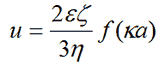
The Henry equation [1] relates the electrophoretic mobility of a particle in solution to its zeta potential:-
|
where ε, ζ, κ, η are the dielectric constant of the dispersant, zeta potential, the inverse Debye length and the viscosity of the dispersant respectively.
Here the function f(Ka) depends on particle shape, but is known for a sphere. The limiting cases of f(Ka), f(0) = 1 and f(∞) = 1.5 correspond to the Hückel and Smoluchowski models respectively.
The White-Mangelsdorf model [2] calculates transport properties by solving the equations of motion of a sphere dispersed in an aqueous ionic system. It models the forces on the particle (the electric field and viscous drag) together with the electrostatic forces between the ions and particle and the electrostatic and drag forces on the ions themselves. It also models the Stern layer as a very thin layer of immobile water, in which ions are free to move. The O'Brien and White [3] model was a precursor to this theory, but did not model the Stern layer.
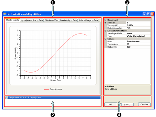
For the purposes of the following discussion, the application in terms of its main constituents is described, namely (1) the Tabbed Graph display, (2) the Graph key, (3) the current Sample Properties and (4)the Command buttons (figure 1).
|
The basic operation of the software consists in defining the sample properties and modeling parameters in the Sample Properties grid control and clicking on the Calculate button. This will plot a graph from the defined set of sample properties and parameters. These sample properties
and parameters can be changed for comparison purposes and a new graph overlaid over the current graph. For each plot generated, a new legend is added to the Graph key list.
The tabbed graph display area consists of a number of plots (figure 1):
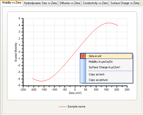
The axis settings can be modified to display the zeta potential and mobility in standard units by using the context menu obtained by clicking on the graph with the right mouse button (figure 2). Note that this menu also allows the copying of the graph contents as text or as a picture which can be copied into, for example, Microsoft Word or Excel.
|
The other graphs can be displayed by selecting different tabs along the top of the graph. These are only available for the White-Mangelsdorf/ O'Brien-White model. For the O'Brien-White model, the graph of surface charge is the total charge behind the slipping plane i.e. equivalent to the total charge in the Stern-Layer and on the particle surface.
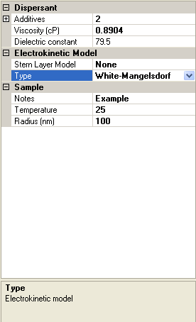
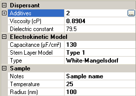
The screen shot in figure 3 shows the Sample property grid. Its appearance will vary depending on which Electrokinetic Model type has been selected, and if White-Mangelsdorf [2] has been chosen, which Stern layer model has been chosen. For all models, Viscosity, Dielectric constant, Sample Notes and Temperature will be visible.
|
The different views obtained by different model selections are discussed in the following sections.
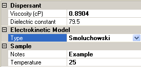
Figure 4 shows which Sample options are available if Smoluchowski is chosen as the electrokinetic model. The choice of Hückel will result in similar looking options, with the model type obviously displaying Hückel rather than Smoluchowski.
|
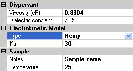
For the Henry model, an extra parameter is required, ka, the product of the inverse Debye length with the particle radius (figure 5). This is a dimensionless parameter, and the Smoluchowski and Hückel models are limiting cases of large and small values of Ka.
|
If the White-Mangelsdorf [2] is chosen as an electrokinetic model, there are additional input parameters (figure 3). These are discussed in the following sections.
This is the radius of the particle and is the equivalent of the hydrodynamic radius in high salt conditions where the Debye length is negligible due to double layer compression.
These parameters will depend on the particular Stern layer model used and if none is used, the model is equivalent to the O'Brien and White model [3]. There are two other options for Stern Layer model type: Type 1 or Type 2. The form of the input parameters is the same for both of these.
If either Type 1 or Type 2 is selected for the Stern Layer model, an extra parameter is included in the sample property grid. This is the Stern Layer capacitance, which essentially determines the potential drop from the Stern Layer to the particle surface (figure 6).
|
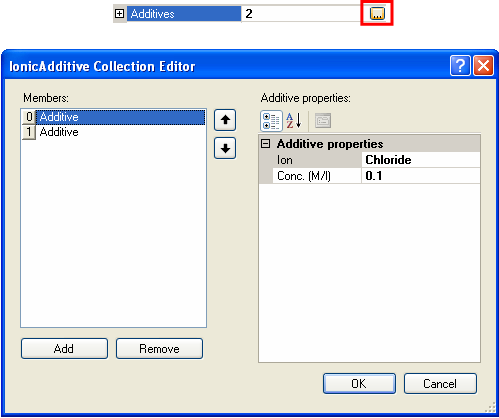
The White-Mangelsdorf model requires information on the concentration and properties of ions in solution. These are entered by selecting the additives section of the sample property grid and clicking on the collection button (the button with ellipses). This will open the Ionic Additive Collection Editor (figure 7).
|
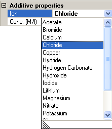
Additives can be added and removed by clicking on the Add and Remove buttons. The selection of what ion "additive is used" can be changed by selecting the relevant ion from the drop down list of available ion species (figure 8). The concentration is the molar concentration of that particular ion. Note that the sum of the additives must be electrically neutral. For example, with monovalent salts, the concentrations must be equal. For more complicated salts, the concentrations used must reflect the stoichiometry of the system.
|
Stern Layer Parameters
There are three possible Stern-Layer model types supported in the electrokinetic utility. The first is not to use a Stern Layer at all - "None". This corresponds to the O'Brien and White model. The other types are "Type 1" and "Type 2", which correspond to free surface binding and specific binding models of ions attaching to the particle surface respectively. Of the two, the "Type 1" is recommended, but both come with the cost of knowing more information about the sample system involved.
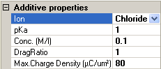
If Type 1 or Type 2 is selected, the additives dialogue is modified (figure 9). As before, the ionic species and concentration of the ionic species must be supplied. In addition, however, the pKa, drag ratio and maximum surface charge density corresponding to that ionic species must be supplied.
|
(i) pKa
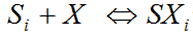
The pKa is the -log10 of the dissociation reaction of a given ionic species Xi onto an empty Stern-layer site Si:-
|
Clearly small (large) K corresponds to weakly (strongly) dissociating systems. See for example http://en.wikipedia.org/wiki/ Dissociation_constant
(ii) Drag Ratio
The mobility of the individual ions is required as part of the calculation, but are well tabulated, and the program knows of these. In the Stern layer, the mobility of individual ions may well be different from the values in free solution. The drag ratio is the ratio of the ionic mobility in the Stern layer to the free solution value. Thus if the values are less (greater) than unity, the ion mobilities are lower (higher) in the Stern layer.
(iii) Maximum Charge Density
This parameter effectively determines the maximum number of free sites available for adsorption. In other words, the maximum density of each individual ionic species that the particle surface will support.
This part of the screen ((2) in figure 2) displays a list of currently displayed plots. They can be removed from the list by selecting and pressing the delete key, or they can be removed from the graph window by clicking off the check box. The parameters used by the active selection are displayed in the property grid display.
The command buttons are located at (4) in figure 2. Clicking on 'Calculate' will generate a new curve (and corresponding data set) based on the current Sample properties. The data set can be saved to a file by clicking on 'Save…' and archived datasets can be loaded from files and re-displayed by using the 'Load…' command.
[1] R.J. Hunter (1981) Zeta Potential in Colloid Science: Principles and Applications. Academic Press, UK.
[2] C. Mangelsdorf and L. White, (1990) J. Chem. Soc. Faraday Trans. 86, 2859.
[3] R. O'Brien and L. White (1978) J. Chem. Soc. Faraday Trans. 77, 1607.