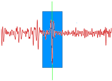
The Morphologi G3-ID particle analysis system obtains chemical identification data for individual particles using Raman spectroscopy. The system's software applies a series of methods to improve chemical identification and measurement robustness.
The chemical analysis part of a Morphologi G3-ID measurement involves a Raman spectrum being acquired from each targeted particle. Acquired spectra are compared with library spectra and a correlation calculation is performed to determine the chemical nature of the targeted particles. A particle spectrum correlation score close to 1 indicates a strong match to the reference spectrum, whereas a score close to 0 means no match to the reference spectrum.
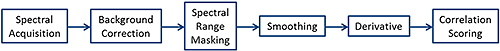
The Morphologi G3-ID software offers a number spectral processing steps in order to improve chemical identification and measurement robustness.
Figure 1 shows the processing steps available in the order that they are carried out.
|
The steps to use depend on the application and the regions of the spectrum of interest. This technical note explains the different options and offers guidance as to which options are appropriate to use for different applications.
A reference library must be created for the correlation to be performed against. This can be updated and data sets reanalyzed against different libraries after Raman acquisition.
Spectra for the library can be acquired in two ways.
For ideal reference libraries, pure samples of the materials should be prepared in the same way as the full formulation.
Acquiring reference spectra in the manual microscope allows optimization of the acquisition time.
The acquisition time required may depend on the Raman scattering efficiency of the materials of interest, the particle size range of interest and the sample preparation method.
If there is more than one component of interest, the acquisition time should be determined by the weakest Raman scatter.
The spot size of the laser with the 50x is approximately 3 µm. Acquisition from smaller particles will have a lower signal to noise ratio, thus the acquisition time needs to be sufficient for the smallest particles of interest. If a wet sample preparation method is used, a longer acquisition time will be required, as the laser has to pass through the coverslip.
|
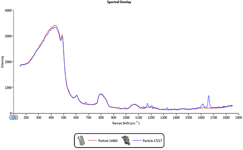
Figure 2 shows an overlay of spectra from a pharmaceutical nasal spray formulation where the blue line is the spectrum from the drug ingredient and the red line is the spectrum from the excipient. The excipient is a very weak Raman scatterer and as a result its spectrum is similar to the background spectrum of the quartz substrate. However, the drug gives strong spectral features in the 1550 cm-1 to 1750 cm-1 region of the spectrum. In this case, it is only the drug component that is of interest so the acquisition parameters should be optimized for this.
Note: If the acquisition times need to be amended, measurements will need to be repeated.
The Morphologi software allows removal of spectral contributions due to the sample substrate (typically high purity quartz) to allow spectral features to be more easily identified for samples which have weak Raman spectra.
Alternatively if the principle spectral features of the material of interest are well defined and well separated from any other features, spectral masking could be used instead of background correction.
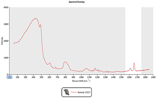
In the nasal spray example, spectral range masking could be used so that the correlation is only carried out over the 1550 cm-1 to 1750 cm-1 region where the features for the drug particles of interest are most prominent. Figure 3 shows the drug spectrum, masked so the correlation calculation will only be performed over the region marked in white and will ignore the shaded region.
|
If background subtraction is preferred there are two options in the Morphologi Software: Simple subtraction and substrate subtraction.
Simple background subtraction is an un-scaled subtraction. The background spectrum used must be acquired with the same spectrometer settings as the measurement. Substrate background subtractionuses a background which is scaled to the signal based on its similarity. The more similar the signal and the background the greater the correction ratio applied. This means that a spectrum that has a lot of background signal in it (for example from very small particles) will be corrected much more heavily than a spectrum with very little background in it (for example from large particles). It also means that the acquisition time for background spectrum can be different from the acquisition time of the sample measurement. The substrate background is appropriate for most applications using the quartz substrates.
|
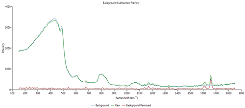
The overlay in Figure 4 shows the raw drug spectrum (blue) (the same as per Figure 2 ), the background spectrum used the correction (green) and the corrected drug spectrum (red).
To reduce noise in the spectrum but preserve the underlying signal savitsky-golay filtering is used (http://en.wikipedia.org/wiki/Savitzky%E2%80%93Golay_smoothing_filter) This process can be thought of as a weighted windowed average where each point on the smoothed signal is calculated by taking a weighted average of the corresponding source value and the values in a window around it. Figure 5 illustrates that the smoothed value for the point of the graph at the green line depends on the values of all of the data points within the blue box; the filter width determines the width of the blue box.
|
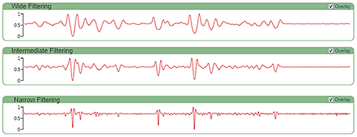
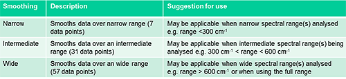
The Morphologi offers three smoothing levels, narrow (over 7 points), intermediate (over 31 points) and wide (over 57 points). The smoothing width determines how many surrounding source values are included in the weighted average.
The option of spectral range masking affects the smoothing, so the level required for this option may be different to when the correlation is performed across the entire spectrum. The signal is smoothed over a window of values on either side and there can be processing artifacts at the ends of the overall signal range (a window of 7 data points will not be able to properly smooth the first and last three data points). Artifacts at the very edge of a spectrum are not an issue for correlation across the whole spectrum, but if spectral range masking is used to reduce the range that data is being processed over, small artifacts can have a more significant effect relative to the total signal.
|
Figure 6 shows an example spectrum with the various smoothing option applied. Choosing narrow smoothing reduces processing artifacts but will increase noise effects throughout the spectrum. More noise in the processed signal with narrower smoothing means the correlation scores will be less robust. In general, it is best to start off with wide smoothing but consider narrower smoothing if spectral range masking is used to exclude a significant portion of the signal.
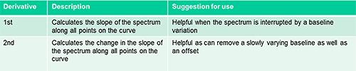
The smoothing option described above determines how much smoothing is applied to spectra, to suppress noise while retaining the signal, before the derivative processing is applied.
The derivative operation produces either the 1st or 2nd derivative of the smoothed signal. The 1st derivative shows the rate of change in the source signal, essentially the angle of the slope of the source signal. The 2nd derivative is the rate of change of the 1st derivative.
|
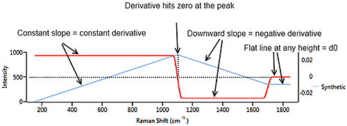
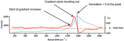
Figure 7 illustrates a synthetic signal (blue) with a rising edge, a blunt peak at 1100 cm-1 then a steady baseline. The derivative (in red) starts at a constant positive value which matches the constant rate of climb of the signal. At the peak of the signal, the derivative drops through zero to a negative value which matches the downward slope of the source signal. When the source signal levels out, the derivative flattens out at zero, regardless of the height of the signal line.
On a real spectrum (soda glass) (Figure 9 ) the spectrum (blue) rises very gently from 200 cm-1 to 1200 cm-1 so the derivative is weakly positive. When the spectrum begins to climb more steeply after 1200 cm-1, the derivative also climbs. As the spectrum levels out near the peak, the derivative drops. At the peak, the derivative is zero then goes negative as the spectrum slopes downward. The downward slope is gentler than the upward slope, so the derivative is less negative than it was positive on the upslope.
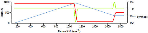
2nd derivative processing applies the derivative operation twice. Figure 8 shows the source spectrum in blue, the 1st derivative in red and the second derivative in green. The green line is showing the rate and direction of change in the 1st derivative.
|
|
This shows that 1st and 2nd derivatives are both effective in determining points of interest in a spectrum where the gradient of the spectrum is changing. 1st derivative is sensitive to a varying baseline whereas the 2nd derivative is less sensitive to broad features in a spectrum.
|
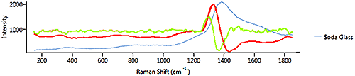
Figure 10 shows the 1st (red line) and 2nd (green line) derivatives of the soda glass signal. The soda glass spectrum has one broad peak and there are no sharp peaks. A 1st derivative would be more appropriate as it is more sensitive to broad features.
|
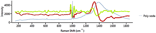
Figure 11 shows a spectrum from polystyrene on soda glass. The 1st derivative in red shows the polystyrene signature peak at just over 1000 cm-1 but gives more weight to the soda glass signature as it is "broader". The 2nd derivative also shows the soda glass signature, but gives more weight to the polystyrene signature because it is "sharper". In this case, if the polystyrene is the component of interest, it is the sharp peak at 1000 cm-1 that is important and using 2nd derivative is more appropriate than 1st derivative.
In general if the material of interest has sharp features, then 2nd derivative is likely to be more effective, whereas 1st derivative is likely to be more appropriate for samples which give a spectrum with broad features
|
|
Figure 12 summarizes guidance as to which processing options should be used for different applications.
The correlation scores can be used to class particles according to the chemical identity. The Morphologi Software allows particles to be classed according to their best correlation to the library spectra or according to specific values, or a combination of both. Once the appropriate combination of spectral processing (background correction, smoothing, processing and spectral range masking) has been applied it is important to look at the spectra of particles with different correlation scores to define which is most appropriate for the specific application.
|
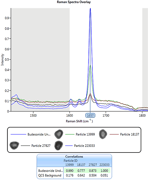
Using the same pharmaceutical nasal spray example from earlier, Figure 13 shows an overlay of the drug library spectrum (blue) and four particle spectra with different correlation scores. For this example, spectral masking has been applied so only the region between 1600 and 1800 cm-1 was included in the correlation. A particle with a correlation score of 0.77 to the drug reference spectrum still gives a distinguishable peak in this region.
For this application particles were classed as being drug if their individual spectrum correlated to the drug library spectrum with a score greater than or equal to 0.7.
In practice the value to use will depend the relative scores of the library component of interest relative to the other components in the library. The more similar the Raman spectra in your library, then the higher the value will need to be to provide correct discrimination. Visual verification of the correct classification of particle Raman spectra is always recommended during method development.