
The Zetasizer series of instruments is operated by analysis software common to the systems. The main function of the analysis is to transform the measured raw data (auto correlation function) into a size result. With the advent of version 6 software there are now three distinct analysis methods available to the user, (1) General Purpose, (2) Multiple Narrow Modes and (3) Protein Analysis [1]. This technical note shows how the same data may lead to slightly different results due to the assumptions about the sample type built into each analysis algorithm. The correlation functions used here are 'ideal' in the sense that they are numerically simulated. Real data are nevertheless expected to follow similar trends.
After a correlation function of the scattered intensity is obtained, in general two different fits are always attempted (1) a cumulants and (2) a distribution analysis.
In the cumulants analysis [2] (according to ISO13321) the logarithm of the correlation function versus delay time is fitted with a linear regression. The emphasis is on the initial time delay channels, and the value of the correlation function below 10% of the initial intercept value is not used (large delay times are simply ignored). The slope leads to a cumulant or z-average size, the curvature leads to a parameter called the second cumulant or polydispersity index, indicative of the overall breadth of the size distribution. For a theoretical Gaussian distribution, the second cumulant is the square of the normalized width at half height. The cumulant method thereby provides an average size and an average sample homogeneity parameter.
In the distribution analysis, no specific assumption about the type of distribution, number of different components, or shape of the distributions is made. A summation of ideal exponential decays is assumed to fit the data, and not just to the initial decay but to larger times (typically 0.01 of the initial intercept). From the infinite range of solutions, a certain solution is selected based on the overall fit and 'smoothness'. For General Purpose, a very conservative smoothness parameter is chosen, where as for Multiple Narrow Mode the choice is more aggressive. In the Protein Analysis, a range of solutions is compared and the best compromise for maximum resolution is then automatically selected [3].
Three sets of data of ten measurements each were generated with the simulation algorithm. The ten measurements were then averaged with the built-in data averaging function. The first was labeled GP for General Purpose, the second set MNM for Multiple Narrow Modes and the third set PA for Protein Analysis. The cumulant result for all three agreed, the mean size was 100.1 nm with a polydispersity index of 0.002. So there is no difference in the cumulants results as would be expected.
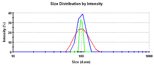
In the intensity distributions, the single peak for this monodisperse sample is broadest for the GP set, followed by the MNM set and narrowest for the PA data. The overlay of the intensity distribution functions is shown in figure 1 with the respective numbers recorded in table 1.
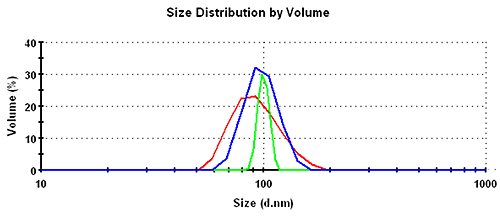
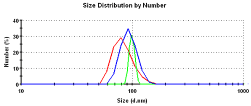
Subsequently, the results in the volume distribution differ as well and are plotted in figure 1. GP shows the lowest mean, followed by MNM, and PA is closest to the nominal simulation size of 100nm. This same trending behavior continues and is even emphasized in the number distributions. The values of the mean and the width for the various analysis schemes and distribution transformations are summarized in table 1.
|
|
|
| Transformation | Analysis | Peak Mean [nm] | Peak Width [nm] | Rel. Width [%] |
|---|---|---|---|---|
Intensity | GP | 104.0 | 23.0 | 23 |
| MNM | 101.5 | 12.9 | 13 | |
| PA | 100.3 | 4.7 | 5 | |
| Volume | GP | 94.5 | 23.4 | 25 |
| MNM | 98.3 | 16.4 | 17 | |
| PA | 99.9 | 5.7 | 6 | |
| Number | GP | 83.7 | 18.3 | 22 |
| MNM | 93.7 | 15.4 | 16 | |
| PA | 99.2 | 5.6 | 6 |
Each regularization analysis scheme has an "inherent" distribution width that limits how narrow a "perfect" size distribution can ever become. This is not a physical limitation set by the distribution itself but is solely due to the mathematics of the inversion algorithms involved. When comparing distributions of different samples it is therefore important to only compare distributions that were obtained under the same mathematical conditions, i.e. to compare only General Purpose or only Protein Analysis distributions from the same set of data. For typical single peak homogeneous distributions the following sequence applies to the width of peaks:
width(GP) > width(MNM) > width(PA)
For the intensity distribution there is a factor of almost 2 between the relative widths of different analysis schemes.
As a rough rule of thumb, good homogeneous and monodisperse samples should be expected to have a relative width in intensity of less than 25%, 15%, or 8% for General Purpose, Multiple Narrow Modes, or Protein Analysis, respectively.
The differences indicate that prior knowledge is required to select the appropriate distribution analysis. If there is no knowledge of the form of the distribution, the General Purpose analysis should be selected. If the distribution is known to consist of a mixture of narrow peaks, Multiple Narrow Modes will give the highest resolution. If the sample is a protein, the Protein Analysis will provide an optimum analysis for a small protein peak in the presence of aggregates.
[1] Software version DTS v6.XX for the Zetasizer Nano series downloadable from the product support area of the Malvern Panalytical website.
[2] ISO 13321:1996 Particle size analysis - Photon correlation spectroscopy
[3] Further details of the regularization algorithm are described in a separate technical note MRK1241-01 "Protein Analysis" downloadable from the Malvern Panalytical resource center.