Cumulants and distribution analyses are algorithms used in dynamic light scattering (DLS) experiments to extract size information from the measured correlogram. The ISO recommended cumulants approach for calculating the mean or z-average size of a distribution of particles from a DLS data set utilizes a moment analysis of the linear form of the measured correlogram. In the cumulant analysis, the 1st cumulant or moment (a1) is used to calculate the intensity weighted z-average mean size and the 2nd moment (a2) is used to calculate a parameter defined as the polydispersity index (PdI).
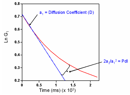
Note from the figure below that the 1st moment is proportional to the initial slope of the linear form of the correlogram and the 2nd moment is related to the inflection point at which log G deviates from linearity.
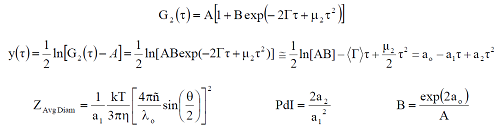
To summarize the above discussion, the cumulants analysis assumes a single particle family and represents the distribution as a simple Gaussian, with the z-average being the mean value and the PdI (polydispersity index) being the relative variance of the hypothetical Gaussian. Note, that for a Gaussian particle size distribution of width (σ) and z-average (X̄), it may be shown that the %Polydispersity from a cumulant fit is σ/X̄ and the PdI is σ2/X̄2 .
Distribution algorithms on the other hand, such as the General Purpose, Multiple Narrow Modes and Protein Analysis, attempt to extract more information, and model the correlogram as an intensity contribution for each of a number of size bands, 70 as a default. These intensities are represented in the displayed size distribution as peaks, each with a characteristic width.
In contrast to the distribution algorithms, which utilize the majority of the exponentially decaying correlogram, the cumulants analysis utilizes only the initial (small delay time values) portion of the correlogram to stabilize the analysis, as using more points will produce unacceptable fit errors. So while we would expect the z-average (derived from cumulants) and Peak 1 (derived from a distribution algorithm) to be similar for a monomodal distribution of particles, small differences are often observed, due to the fact that the cumulants and the distribution algorithms utilize different mathematical approaches to the analysis. The trade off is that the cumulants analysis tends to give a more repeatable mean value, but is unsuitable for a polydisperse sample, i.e. one with a wide single mode, or with a number of different populations. At PdI values > 0.25, it is likely that the z-average mean will not coincide with the mode of the largest peak in the distribution. The distribution algorithm result can provide more information, but requires better quality data to produce a repeatable result.
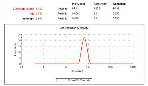
Consider the figure below, which shows the cumulants derived z-average, along with, in this example, the General Purpose derived distribution and corresponding peak mean values, for a latex sizing standard with a hydrodynamic diameter of 62 ± 3nm. As noted in this figure, the ISO recommended z-average of 64nm is within the stated specification range of the sizing standard, whereas the Peak 1 average is slightly higher at 67nm, suggesting that the Peak 1 value might be in error. However, the Peak 1 “width” of 16nm is equivalent to 23% polydispersity (Pk1 width/Pk 1 mean), indicating the likelihood of a small amount of oligomerized or slightly aggregated sample, i.e. for a purely monomeric sample, one would expect a %polydispersity of <15 to 20%. Since the reported Peak 1 value is the mean of the peak derived from General Purpose, it is not surprising that the calculated value is slightly larger than the ensemble average derived from the cumulants analysis.