
This white paper takes you through ITC principles and gives details and tips on a broad application range from studies of a simple 1:1 interactions to complex binding mechanisms and linked equilibria.
Isothermal titration calorimetry (ITC) is an analytical technique that has become the “gold standard” for studying intermolecular interactions. As its name indicates, it is a titrimetric technique, that is, a volumetric laboratory method for quantitative chemical analysis (traditionally intended to determine the unknown concentration of an identified analyte) where a reagent solution, the titrant, is made to react with a solution of analyte or titrand. The ITC instrument measures the heat produced or consumed by the interaction reaction along the titration to determine the endpoint (related to the interaction stoichiometry). By performing the titration at constant temperature and pressure, a single ITC experiment provides information on the equilibrium association constant, the binding enthalpy and the stoichiometry, from which the Gibbs energy and the entropy of binding can be readily calculated. Thus, a single ITC experiment gives direct access to the main thermodynamic potentials associated with the interaction process: Gibbs energy, enthalpy and entropy.
The high sensitivity of modern ITC instruments allows monitoring the formation of non-covalent complexes where molecules interact through a combination of multiple weak interactions: hydrogen bonds, electrostatic interactions, van der Waals interactions, and hydrophobic interactions, mainly. Then, it is possible to study the interaction between any type of molecules from ions and polymers to nanoparticles and biomolecules. Much of the ITC applications are focused on biomolecular interactions, such as the formation of well-defined protein-ligand, protein-protein, protein-DNA, protein-membrane, or DNA-ligand binding complexes (1, 2).
ITC allows a comprehensive quantitative description of a given interaction by providing valuable information at different levels: 1) whether or not two given molecules interact; 2) the binding stoichiometry; 3) the binding affinity or strength of the complex formation through the association/dissociation constant and the binding Gibbs energy; and 4) the partition of the Gibbs energy of binding into enthalpic and entropic contributions. For a biomolecular interaction careful analysis of the experimental results, together with a well-planned set of experiments under different experimental conditions, provides additional information for further characterizing the interaction and addressing: 1) possible conformational changes coupled to the binding process; 2) additional concomitant association/dissociation processes (e.g. net exchange of protons and other ions, as well as water molecules) coupled to and modulating the binding process; and 3) cooperativity phenomena involving homotropic (same ligand) or heterotropic interactions (a different ligand). Thus, ITC gives access to direct information on the interaction, and also on the regulation and modulation of the biomolecular interaction.
A given molecule (usually termed “macromolecule”, M) will have several binding sites for another given molecule (usually termed “ligand”, L). That distinction does not make any assumption on the nature and size of these interacting molecules. Here we will review the thermodynamic background for ITC experiments and its application with a special focus on the simplest system (a macromolecule with single ligand binding site, i.e. 1:1 stoichiometry), with the goal of extracting the maximal amount of information. A great majority of experimental cases found in the literature correspond to that simple system; the description of more complex systems (non 1:1 interaction) can be easily found in the literature (3). In addition, specific details about the instrumentation and experimental protocols can also be found in the literature (4, 5).
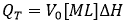
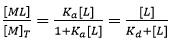
ITC complies with the standard requirements for an experimental technique aimed at studying binding interactions: 1) the observable property must exhibit different values at the different ligated states; and 2) the measured signal must be proportional to the advance of the process. ITC directly measures the heat taking place in a reaction process at constant pressure, QT, which is proportional to the molar enthalpy change associated with that process, ΔH (taking the non-ligated state as a reference), and the amount of macromolecule-ligand complex formed:
 (1)
(1)
|
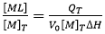
where V0 is the volume of the calorimetric cell, and [M]T is the total concentration of macromolecule in the cell. The first condition means that the enthalpy of interaction (i.e. enthalpy for complex formation) must be different from zero. The enthalpy of interaction is dependent on temperature and other experimental variables (e.g. pH, ionic strength, co-solute concentration), and, therefore, it will be reasonably easy to find a given set of experimental conditions where it is not zero. The second condition is automatically fulfilled from the first condition, since QT is proportional to advance of the binding process (indicated as saturation fraction of macromolecule or molar fraction of complex):
 (2)
(2)
|
Equations 1 and 2 can be used in a model-free fashion for estimating the binding enthalpy, provided that: 1) almost complete saturation of the macromolecule is achieved ([ML]/[M]T close to 1); 2) appropriate subtraction of the reference background heats is performed; and 3) protein concentration is determined with reasonable precision.
Compared to other biophysical techniques to study binding interactions, the main advantages of ITC are: 1) complete basic thermodynamic characterization (stoichiometry, association constant, and binding enthalpy) in a single experiment; 2) heat is a universal signal, and, therefore, there is no need for reporter labels (e.g. chromophores, fluorophores); 3) direct determination of the binding enthalpy (no need for additional assumptions regarding the van’t Hoff relationship); 4) non-destructive technique; 5) interaction in solution (no need for reactant immobilization); 6) possibility of performing experiment with optically dense solutions or unusual systems (e.g. dispersions, intact organelles or cells); and 7) relatively fast (from 0.25 h/assay in the single injection experiment to 2 h/assay in the conventional titration experiment).
Of course, some disadvantages can be pointed out for ITC: 1) signal is proportional to binding enthalpy, and non-covalent complexes may exhibit rather small binding enthalpies (normally, │ΔH│ < 40 kcal/mol, but in the majority of cases │ΔH│ < 25 kcal/mol); 2) heat is a universal signal, and every process will contribute to the global measured heat, thus complicating the evaluation of the contribution due to binding; 3) a large amount of sample required, but this has been reduced significantly (e.g. ~ 0.04 – 1 mg/assay for a 50 kDa protein); 4) it is a slow technique with a low throughput (0.25 – 2 h/assay), not suitable for HTS; 5) kinetically slow processes may be overlooked; 6) a limited range for reliably measured binding affinities (association constants from 104 – 109 M-1 for the conventional titration experiment); and 7) until recently no kinetic information for binding interactions was accessible.
Many of these disadvantages are not restricted to ITC and are shared between many other binding techniques. In addition, some of them can be overcome or minimized. For example, buffers with low ionization enthalpy can be employed for reducing buffer-dependent unspecific de/protonation effects contributing to the measured enthalpy, and extreme care should be taken when dissolving/solubilizing reagents to guarantee a composition match between all solutions in order to reduce the background injection heat (also called “dilution heat”). In addition, the practical range for affinity determination can be extended by performing displacement titrations, and new methodologies for estimating reliable kinetic information on the binding have been recently developed (6, 7).
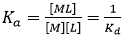
When a macromolecule with a single binding site and a ligand are mixed at certain experimental concentrations, the extent of the reversible binding reaction, that is, the concentration of the macromolecule-ligand complex, [ML], is governed by the equilibrium association constant, Ka, which is given by:
 (3)
(3)
|
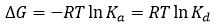
where Kd is the equilibrium dissociation constant for the complex, [M] and [L] are the concentrations of free macromolecule and ligand. Both equilibrium constants are related to the (standard) Gibbs energy of binding, ΔG:
 (4)
(4)
|
where R is the gas constant and T the thermodynamic or absolute temperature. The larger the association constant, the smaller dissociation constant and the more negative the Gibbs energy of binding, resulting in a stronger complex.
From Eq. 3 it is obvious that if [L] = 1/Ka = Kd, the macromolecule is equally distributed into the free and liganded states. Eq. 3 leads to the well-known hyperbolic relationship between the molar fraction of macromolecule-ligand complex and the concentration of free ligand:
 (5)
(5)
|
from which the concentration of macromolecule-ligand complex formed and, therefore, the heat associated with that formation could be readily calculated just by multiplying by the total concentration of protein and the molar binding enthalpy. Unfortunately, in a titration experiment the concentration of free ligand is unknown and the controlled concentrations are the total concentration of macromolecule and ligand. Therefore, Eq. 5 cannot be employed in the analysis of the titration.
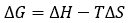
The binding Gibbs energy can be partitioned into its enthalpic, ΔH, and entropic, -TΔS, contributions:
 (6)
(6)
|
The basic thermodynamic binding profile for a given interaction consists of the three main binding parameters, Gibbs energy (calculated from the equilibrium association constant Ka), enthalpy and entropy of binding. The combination of these three thermodynamic potentials provides valuable and fundamental information on the binding process (e.g. what type of intermolecular interactions drive the interaction).
Despite the relation between the thermodynamic potentials, binding affinity (either in the form of equilibrium constants or Gibbs energy of binding) is not correlated with enthalpy of entropy of binding. That is, high affinity or low affinity is not necessarily associated with a certain distribution of affinity into the enthalpic and entropic contributions. Thus, two ligands with similar affinity may exhibit markedly different thermodynamic binding profiles in which one of them shows an enthalpically driven binding (enthalpic contribution is negative, favorable to binding, and entropic contribution is positive, unfavorable to binding), while the other ligand shows an entropically driven binding (enthalpic contribution is positive, unfavorable to binding, and entropic contribution is negative, favorable to binding).
An important aspect is that the basic thermodynamic profile is dependent on temperature and other environmental variables (e.g. pH, ionic strength) and, consequently, it will be important to assess such dependency in order to predict the behavior of the macromolecule-ligand complex under different environments (e.g. a physiological protein-protein complex that is intracellularly subjected to acidification of its environment). Structural alterations in the binding partners (e.g. mutations in the binding protein, functional derivatives of the ligand) will also modulate the thermodynamic binding profile as well.
Basically, the main goal in a titration experiment is to determine equilibrium association constant, the binding enthalpy and the stoichiometry and, thus, the thermodynamic profile, as well as its dependency on environmental variables and structural changes in the binding partners (if possible).
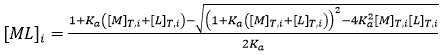
As indicated before, a single ITC experiment provides the complete basic thermodynamic profile for a given binding interaction. The experimental methodology consists of performing a series of injections of titrant (usually the ligand) from a syringe into the titrand solution (usually the macromolecule) in the cell in a completely automated fashion, while keeping the system under quasi-isothermal, isobaric conditions. By injecting the ligand sequentially, the chemical equilibrium is perturbed by the incremental changes in the reactant concentrations triggered by the ligand injections, and the system goes through a set of equilibrium states differing in their composition, since the partition between free macromolecule and ligand-bound macromolecule depends on the equilibrium (association or dissociation) constant and the total concentrations of macromolecule and ligand:
 (7)
(7)
|
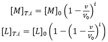
where the subscript i indicates the number of injection along the titration, and the total concentrations of macromolecule and ligand after each injection are given by:
 (8)
(8)
|
where [M]0 and [L]0 are the initial macromolecule concentration in the cell and the concentration of ligand in the syringe, respectively, v is the injection volume, and the (1-v/V0) factor accounts for the dilution taking place in a calorimetric cell operating at constant volume. Each transition between two successive states, triggered by ligand injection, is accompanied by release or absorption of heat (at constant pressure, related to the global enthalpy change) that is proportional to the change in the concentration of complex due to that injection and the molar enthalpy:
 (9)
(9)
|
from which it is clear that ITC is an incremental or finite-difference technique. The heat associated with a given injection in Eq. 9 has been normalized by the number of moles of ligand injected dividing by v[L]0. Figure 1 illustrates a typical calorimetric titration for a macromolecule with a single ligand binding site. Non-linear regression analysis of the experimental data by using Eq. 9 allows the estimation of the equilibrium association constant, the binding enthalpy and the stoichiometry, from which the Gibbs energy and the entropy of binding can be readily calculated. Simple models, like the one considered here, can be handled with fitting routines provided by the instrument manufacturers.
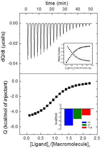
|
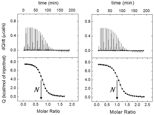
Even for this simple system with a single ligand binding site, it is usual to include an additional parameter N multiplying [M]0 in Eq. 8 or [M]T,i in Eq. 7. This parameter will represent either the stoichiometry (in a model for a macromolecule with N identical and independent binding sites, that is, the “one set of binding sites” model) or the fraction of active (binding competent) macromolecules with a single ligand binding site. Very often ITC titrations are the best way to estimate the concentration of (active) macromolecule, because standard methods (e.g. UV absorption, colorimetric methods, elemental analysis) are either affected by systematic errors or they just provide total concentration of protein, with no distinction between functional and non-functional macromolecule (e.g. misfolded protein). Thus, fractional values of N may be due to uncertainties in both reactant concentrations. Usually, ligand concentration can be precisely determined if spectroscopic data and/or accurate weighing procedures are available, and they are not prone to fast degradation; however, even if extreme care is taken, it is not unusual to end with a significant fraction of protein in a non-binding competent conformation. Therefore, it is possible to normalize the nominal protein concentration using the parameter N in order to get a non-fractional N value (Figure 2), thus “titrating” the protein solution (that is, determining its correct concentration from the known concentration of a reactant). Furthermore, because the binding enthalpy estimate is mostly dependent on the ligand concentration in the syringe, whereas the normalization factor N is dependent on both concentrations, in principle, knowing the expected value for the binding enthalpy it will be possible to estimate both reactant concentrations from a single titration: ligand concentration is estimated using the binding enthalpy, and, later, macromolecule concentration is estimated using N. When studying a given protein, it is very convenient to have a calibrating ligand for which binding parameters are known with reasonable accuracy, useful for quality control in protein production stages.
|
In order to correctly apply Eq. 9 in the analysis of an experimental titration and obtaining good estimates of the binding parameters, the “heat of dilution” problem must be addressed. Besides the heat associated with the macromolecule-ligand interaction, the injection of ligand solution into the cell may be accompanied by a non-negligible amount of background heat, potentially due to dilution of the ligand, the mechanical effect of the injection (e.g. turbulence, mixing), or equilibration of small mismatches in composition between titrant and titrand solutions (e.g. small differences in pH, DMSO or glycerol concentration when these additives are required). There are three ways to remove the contribution this unspecific heat effect: 1) performing a control experiment by diluting ligand into buffer and subtracting the resulting heats from the ligand-macromolecule titration; 2) averaging the heats associated to the last injections (close to macromolecule saturation) in the ligand-macromolecule titration and subtract that value from the data; and 3) introducing in Eq. 9 an additional adjustable parameter, Qd, accounting for the injection background heat. The third option is the preferred one, because the dilution experiment does not necessary properly mimic the injection background effect when macromolecule is present (subtraction of control experiment from titration may not give satisfactory results), and very often macromolecule saturation is not completely achieved (average of heats associated with last peaks may be meaningless, as shown in Figure 1). Apart from this, it is critical to routinely perform control experiments (e.g. diluting ligand into buffer in order to rule out unexpected phenomena, such as ligand self-association), as well as calibration test, either performed electrically or, preferentially, chemically (by using well-characterized standard chemical processes).
Efforts towards miniaturization and automation of laboratory instruments has made available ultrasensitive calorimeters, such as MicroCal™ Auto-iTC200, suitable for accurately measuring reaction heats per injection of a few microcalories starting from a fraction of a mg (dozens of micrograms) of material in the calorimetric cell. Their simplicity, reliability and accuracy have made calorimetric titrations to become a standard technique, many times the preferred one, for biophysical interaction studies.
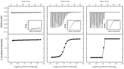
In principle, from a single titration it is possible to estimate the equilibrium association constant, the binding enthalpy and the stoichiometry. However, the reliability of that determination depends on the binding affinity and the experimental set-up. A dimensionless parameter c = Ka[M]0 = [M]0/Kd can be calculated, and: 1) if 1 < c < 10000, the three binding parameters can be simultaneously and accurately estimated; 2) if c > 10000, only the binding enthalpy and the stoichiometry can be determined; and 3) if c < 1, only the equilibrium association constant can be determined, since the binding enthalpy and the stoichiometry will be correlated (but, if N can be fixed during the regression analysis and sufficient macromolecule saturation is reached, the binding enthalpy can also be reliably determined). The indicated range for reliable binding affinity estimation (1 < c < 10000) is fairly generous; although c values somewhat larger than 1000 usually do not represent a problem for binding affinity estimation, the optimal range is 10 < c < 1000. Figure 3 illustrates the three different scenarios according to the value of c. Interestingly the best scenario correspond to performing a titration using a macromolecule concentration much larger than the equilibrium dissociation constant Kd; however, in a standard spectroscopic titration (e.g. fluorescence, NMR, circular dichroism…) it is advisable to employ a macromolecule concentration around the Kd value for optimal results.
|
Since the curvature of the titration depends on the parameter c, given a binding affinity, it could be possible to modulate that curvature by selecting the macromolecule concentration. Though the best situation is that of 1 < c < 10000, it is not always possible to work within this window, because we might end using very low reactant concentrations (if the binding affinity is very high), which is conducive to a low calorimetric signal, or using prohibitively high reactant concentrations, resulting in a large calorimetric signal (out of the instrumental range) or concentrations far from being practically feasible.
In case our experimental system exhibits very high (c > 10000) or very low (c < 1) affinity, displacement titrations including a moderate affinity ligand make it possible to overcome that difficulty (8).
Because enthalpy and entropy of binding reflect interaction of very different nature, the thermodynamic binding profile provides valuable information on the interatomic interactions underlying the binding event and on the mode of interaction between macromolecule and ligand. The enthalpic contribution mainly reflects specific interactions between the two reactants (formation of hydrogen bonds, van der Waals, electrostatic and hydrophobic interactions), while the entropic contribution reflects unspecific interactions between macromolecule and ligand (desolvation of the binding interface, geometric complementarity between ligand and macromolecule binding site, as well as structural rigidity of the ligand). Therefore, it is possible to establish that enthalpically driven ligands bind to the macromolecule because they interact specifically with the target (i.e. they “like” to be in the binding site), whereas entropically driven ligands bind to the macromolecule because they are very hydrophobic and have the appropriate geometry and structural rigidity (i.e. they “do not like” to be in water).
It is important to emphasize that these changes in the thermodynamic potentials associated with the binding event not only reflect the creation of a considerable network of intermolecular interactions (e.g. hydrogen bonds, van der Waals interactions, electrostatic interactions, hydrophobic interactions) between macromolecule and ligand, but also the disruption of rather similar interactions of both molecules with the solvent molecules. Therefore, these changes are the net result of competing interactions where the solvent molecules play an important role. Globally the binding affinity is the net result of these different enthalpic and entropic contributions.
Besides the valuable information on the mode of binding between macromolecule and ligand, the partition on the Gibbs energy into enthalpic and entropic contributions has important consequences. It has been established that the Gibbs energy of binding is rather insensitive to alterations in the environmental variables and alterations in the binding partners. This last statement is closely related to the enthalpy-entropy compensation (i.e. changes in the enthalpic contribution to the binding are generally coupled to opposing changes in the entropic contribution, thus keeping the Gibbs energy of binding almost unaltered) and the difficulties for improving the ligand binding affinity by engineering the ligand structure. However, it is found that the Gibbs energy temperature-derivative related potentials (that is, enthalpy and entropy of binding) are more sensitive to environmental variables and alterations in the binding partners, resulting in binding parameters more amenable to interpretation. Evidences have been found suggesting that the distribution of the Gibbs energy into its enthalpic and entropic contributions has important consequences regarding the optimization of ligand binding affinities and the minimization of the susceptibility of ligands to structural changes (either induced by mutations or due to natural variability) in the macromolecular target (9, 10).
A given macromolecule may interact with more than one ligand. In the particular case of a macromolecule interacting with two different ligands, besides characterizing the binding interactions for each ligand with the macromolecule, when no structural information is available, it would be interesting to assess whether or not the ligands bind competitively (either directly by binding to the same binding site, or indirectly through a conformational change that precludes the binding of the second ligand). ITC is particularly appropriate for this evaluation, because, contrary to other techniques in which only one binding parameter (binding affinity) is employed for discriminating between independent, cooperative or competitive binding, in ITC we can use two binding parameters (binding affinity and enthalpy) for discriminating the three scenarios.
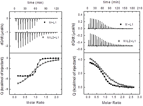
The set-up for this experimental procedure is rather simple: 1) perform two titrations by injecting each ligand into macromolecule; and 2) perform a third titration by injecting one of the ligands into the macromolecule pre-bound to the second ligand (second ligand in excess, if possible). All titrations, binary and ternary, can be analyzed with the single binding site model (if ligand 2 is in excess regarding the macromolecule concentration, the ternary titration can be analyzed as a binary titration). Then, three sets of binding parameters (equilibrium constant and binding enthalpy) can be obtained from all three titrations: Ka,1 and ΔH1 for ligand 1 interaction, Ka,2 and ΔH2 for ligand 2 interaction, and Ka,12 and ΔH12 for ligand 1 interaction in the presence of ligand 2. The discrimination between the different scenarios is based on a comparison of these three sets of parameters. As we will see, because independent binding and competitive binding are special limiting cases of cooperative binding (in particular, competitive binding is the limiting case for maximal negative cooperativity), we will discuss the general cooperative case, and then we will particularize to the competitive and independent cases.
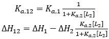
If the two ligands bind cooperatively, the apparent binding parameters for ligand 1 in the presence of ligand 2 (at a certain concentration) are:
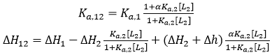 (14)
(14)
|
where [L2] is the free concentration of ligand 2 in the calorimetric cell (if ligand 2 is employed at a total concentration much larger than that of the macromolecule, its free concentration can be approximated by its total concentration), α is the cooperativity interaction constant (0 < α < 1 corresponds to negative cooperativity, and 1 < α < +∞ corresponds to positive cooperativity), and Δh is the cooperativity binding enthalpy. Eq. 14 provides the apparent binding parameters for ligand 1 interacting with the macromolecule in the presence of ligand 2 at a certain concentration. However, the intrinsic binding parameters for ligand 1 interacting with the macromolecule pre-bound to ligand 2 are different: if ligand 2 is bound to the macromolecule, ligand 1 interacts with the macromolecule with an intrinsic equilibrium association constant αKa,1, and an intrinsic binding enthalpy ΔH1 + Δh (i.e. saturating concentrations of ligand 2 in Eq. 14).
If the two ligands bind independently, the binding of ligand 2 to the macromolecule in the ternary titration will not affect the outcome of the titration, and, then, α = 1 and Δh = 0:
 (15)
(15)
|
If the two ligands bind competitively, the binding of ligand 2 to the macromolecule in the ternary titration will block the binding of ligand 1, and, then, α = 0:
 (16)
(16)
|
Therefore, once the three sets of binding parameters are obtained from the analysis of the binary and ternary titrations, we must apply consecutively the previous equations as discriminating criteria, starting from the independency test (Eq. 15), followed by the competitiveness test (Eq. 16). If none of these tests is fulfilled, taking into consideration the experimental uncertainties in the estimated binding parameters, then the two ligands bind cooperatively (i.e. neither independently nor competitively). Figure 4 illustrates this procedure in two experimental systems.
|
It has been stressed before that the enthalpic and entropic contributions provide fundamental information on the binding interaction. Because the entropic contribution is calculated from the estimated binding enthalpy and Gibbs energy, it is extremely important to get good estimates of those binding parameters and eliminate possible extrinsic contributions.
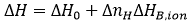
A potential contribution to the Gibbs energy and the enthalpy of binding comes from the exchange of protons upon binding between the macromolecule-ligand complex and the bulk solution. If certain ionizable groups (from any of the two binding partners) undergo a pKa change due to a change in its solvent exposure as a result of the ligand binding (either by direct binding or induced by the conformational change), then, there will be a change in the proton fraction saturation between each ionizable group in the free reactants and in the complex. This will result in a net proton exchange (uptake or release) which will be balanced by the buffer in order to maintain a constant pH, resulting in a contribution of the buffer Gibbs energy and enthalpy of ionization to the overall binding parameters. Fortunately, if the selected buffer has a pKa similar to the experimental pH, the measured Gibbs energy of binding will not contain a significant contribution from the buffer ionization process. On the contrary, if the selected buffer has a considerable ionization enthalpy, ΔHB,ion, the measured enthalpy of binding, ΔH, might contain a significant contribution from the buffer ionization process:
 (12)
(12)
|
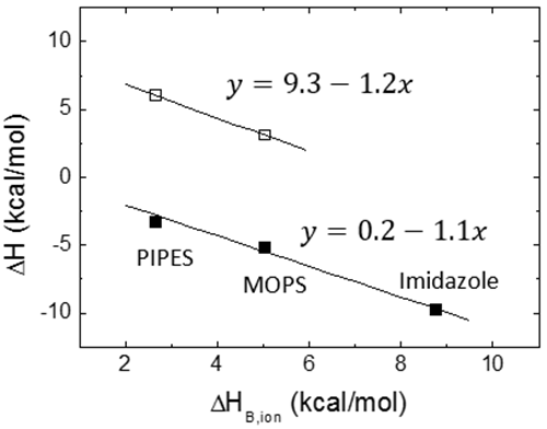
where ΔH0 is the buffer-independent binding enthalpy, and ΔnH is the net number of protons exchanged between the complex and the bulk solution as a result of ligand binding. The parameter ΔnH may get non-integer values, since it is a statistical parameter accounting for the difference in the global proton fraction saturation between the free reactants and the complex; it indicates a net protonation of the complex when positive, and a net deprotonation of the complex when negative. It is clear that the contribution from the buffer in Eq. 12 may dominate the global measured binding enthalpy, which could be inappropriate for determining the ligand binding enthalpy, but sometimes may be advantageous for amplifying the calorimetric signal when the ligand binding enthalpy is low. According to Eq. 12, performing ITC experiments at the same conditions (temperature, pH, ionic strength,…) and using buffers with different ionization enthalpies, it is possible to assess proton exchange processes coupled to ligand binding and estimate the buffer-independent binding enthalpy (to reliably establish the thermodynamic binding profile with no extrinsic contributions to the binding) and the net number of protons exchanged. Figure 5 illustrates this experimental procedure. Alternatively, it is possible to employ buffers with very low or negligible ionization enthalpy (e.g. phosphate or acetate) and determine the buffer-independent binding enthalpy in a single experiment, with no need to apply Eq. 12. As a corollary, it is important to point out that there are no bad buffers in calorimetry: the buffer may distort and largely modulate the observed binding enthalpy (if proton exchange processes take place upon binding and the ionization enthalpy of the buffer is large enough), but that might help in detecting the interaction by amplifying the heat signal and there is a procedure to remove its contribution to the measured enthalpy.
|
Interestingly, from the value of ΔnH we can predict the behavior of the binding affinity with a change in pH. If ligand binding is coupled to proton exchange processes, the thermodynamic binding profile will be pH-dependent; in particular, according to a well-known chemical linkage relationship, the equilibrium association constant and the Gibbs energy of binding will be pH-dependent:
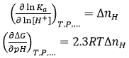 (13)
(13)
|
Knowing ΔnH from experiments performed at a constant pH and using Eq. 12, we may quantitatively predict the change in binding affinity for finite changes in pH (within a limited pH variation range, e.g. |ΔpH| ≤ 2 ); in particular, if ΔnH > 0 (net complex protonation) the binding affinity will decrease with pH, and if ΔnH < 0 (net complex deprotonation) the binding affinity will increase with pH.
The heat capacity of binding (at constant pressure) is the temperature derivative of the binding enthalpy:
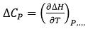 (10)
(10)
|
which is easily accessible experimentally by performing titrations at different temperatures and plotting the observed experimental binding enthalpy as a function of temperature; within a small temperature range (e.g. 10-40°C), the observed binding enthalpy often exhibits a linear trend, from which the binding heat capacity is estimated as the slope of the linear regression.
The binding heat capacity is strongly connected with the burial and desolvation of binding interfaces. The reduction in accessible surface area in the macromolecule and the ligand, with contributions from dehydration of polar and apolar regions, leads to a reduction in the system heat capacity (capability of storing and exchanging thermal energy): the dehydration of polar regions makes the heat capacity more positive, whereas the dehydration of apolar regions makes the heat capacity more negative, the latter being predominant in binding interfaces though. Other phenomena (e.g. reduction in local mobility and vibrational degrees of freedom in the macromolecule and the ligand) also contribute to the heat capacity of binding, but to a lesser extent (<10%). The connection between binding heat capacity and reduction in (polar and apolar) accessible surface area upon complex formation has made possible to establish linear relationships between both quantities, the first one accessible through ITC and the second one through structural techniques (e.g. X-ray diffraction, NMR).
The success of this structural parameterization of the binding heat capacity has enabled the assessment of potential conformational changes coupled to the ligand binding event from the structural information of the complex, even in the case the structures of the free binding partners are not available. Assuming a rigid-body complex formation with no conformational change, the structures of the free binding partners can be directly obtained from the structure of the complex and the changes in (polar and apolar) accessible surface area can be calculated. From those changes, the binding heat capacity corresponding to the rigid-body binding interaction can be estimated. The deviation of the calculated binding heat capacity from the experimentally determined binding heat capacity is directly related to the extent of the possible conformational change coupled to ligand binding.
As it has been indicated above, the observed binding enthalpy usually exhibits a linear behavior within a limited temperature range. In some cases this is not true, and a curved trend with a variable slope appears (gradually more negative slope as temperature increases), which implies a temperature dependent binding heat capacity. This occurs when the conformational change coupled to binding is coupled to a temperature dependent conformational equilibrium within the operational temperature range: the simplest explanation is that one of the binding partners exhibits an equilibrium between two conformations, native and partially unfolded conformations, and the increase in temperature gradually shifts the equilibrium towards the non-native conformation; then, a gradual transition from a small binding heat capacity (ligand binding to the native conformation) to a large one (ligand binding to the non-native partially unfolded conformation) is observed. Globally, there is a temperature-induced conformational change opposing a ligand-induced conformational change, and the temperature-dependent conformational change is the one responsible for the curvature in the enthalpy plot.
As a corollary, some words about conformational changes coupled to ligand binding. If no conformational changes occur upon ligand binding, a linear trend should be observed in the measured binding enthalpy vs. temperature plot. However, this is not a sufficient condition: a linear trend in that plot is not an indication for the absence of conformational changes coupled to ligand binding. Thus, a linear trend in the binding enthalpy will indicate that the conformational change, if any, occurs at the same extent along the experimental temperature range (roughly the same shift in the populations of the conformational states, irrespective of the temperature; or, in other words, there is no temperature-dependent conformational equilibrium). If the conformational change occurs at a different extent in a temperature-dependent manner within the experimental temperature range (different shift in the populations of the conformational states, depending on the temperature, or, in other words, there is a temperature-dependent conformational equilibrium modulated by ligand binding), then, a curved plot with variable slope will be observed for the measured binding enthalpy.
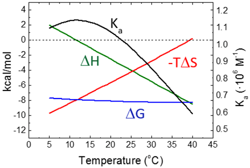
In addition, the binding heat capacity allows extrapolation of the binding thermodynamic potentials (Gibbs energy, enthalpy and entropy of binding) obtained at a certain reference temperature T0 within a given temperature range to evaluate the behavior of the binding affinity with a change in temperature:
 (11)
(11)
|
Figure 6 shows the temperature dependency of the thermodynamic binding profile for a given binding interaction, assuming a constant binding heat capacity.
|
Advances in ITC instrumentation (automation, miniaturization) have made available an automated high-throughput ITC, MicroCal Auto-iTC200, allowing low sample/time consumption per experimental assay (~50 assays/day). Additional methodological developments, like the single injection method, may increase significantly the throughput, while maintaining the accuracy (11).
ITC is a powerful technique for characterizing interactions, in particular, interactions of biomolecules within a broad range of binding affinities (from the characteristic low affinities typical in physiological mechanisms, to the very high affinities found in drug design and development stages).
Among the many fields and application where ITC can play a key role, we may highlight: 1) protein function and regulation, characterizing mode of interaction, specificity, and allosteric interactions (e.g. enzymatic mechanism, receptor signaling); 2) protein engineering and function redesign; 3) characterization of pharmacological/biotechnological targets; 4) selection of leads in drug discovery; 5) optimization of leads in drug development, according to a quantitative-structure-energetic-activity relationship; 6) development of drug carriers for improved therapeutic administration; 7) pre-clinical assays (e.g. plasma protein binding, potential side-effects through unwanted targets); 8) experimental benchmark for development and refinement of computational models for protein interactions (docking, virtual screening, prediction of interaction energetics,…); and 9) quality control for protein/biologics production in pharmaceutical, cosmetic, food, cleaning and biotech industry.
This white paper is authored by Dr. Adrian Velazquez-Campoy, currently employed as an ARAID Foundation Researcher at the Institute of Biocomputation and Physics of Complex Systems (University of Zaragoza), Mariano Esquillor s/n, 50018, Zaragoza, Spain. email: adrianvc@unizar.es
Falconer, R.J. and Collins, B.M. Survey of the year 2009: Applications of isothermal titration calorimetry. J. Mol. Recognit. 24, 1-16, (2011).
Ghai, R. et al. Applications of isothermal titration calorimetry in pure and applied research - Survey of the literature from 2010. J. Mol. Recognit. 25, 32-52 (2012).
Vega, S. et al. A unified framework based on the binding polynomial for characterizing biological systems by isothermal titration calorimetry. Methods, in press (2015).
Doyle, M.L. Titration microcalorimetry. Curr. Protoc. Prot. Sci. Unit 20.4 (2001).
Lewis, E.A. and Murphy, K.P. Isothermal titration calorimetry. Methods Mol. Biol. 305, 1-15 (2005).
Sigurskjold, B.W. Exact analysis of competition ligand binding by displacement. Isothermal titration calorimetry. Anal Biochem. 277, 260-266 (2000).
Burnouf, D. et al. kinITC: A new method for obtaining joint thermodynamic and kinetic data by isothermal titration calorimetry. J. Am. Chem. Soc. 134:559-565 (2012).
Velazquez-Campoy, A. et al. Isothermal titration calorimetry. Curr. Protoc. Cell Biol. Unit 17.8 (2004).
Freire, E. A thermodynamic approach to the affinity optimization of drug candidates. Chem. Biol. Drug Des. 74, 468-472 (2009).
Freire, E. Isothermal titration calorimetry: Controlling binding forces in lead optimization. Drug. Discov. Today Technol. 1, 295-299 (2004).
Markova, N. and Hallén, D. The development of a continuous isothermal titration calorimetric method for equilibrium studies. Anal. Biochem. 331, 77-88 (2004).