
Guidance for using the HYDRO SIGHT demonstration software
The Hydro Sight software demo version enables you to see how the imaging accessory may help you with method development or trouble shooting.
The Hydro Sight is an imaging accessory for laser diffraction that is placed in-line between the optical bench and a wet dispersion unit allowing users to see their dispersion. It is designed to help with method development and troubleshooting, building on the Mastersizer 3000 commitment to help our customers achieve Smarter Particle Sizing.
|
The Hydro Sight software demo version enables you to see how the imaging accessory may help you with method development or trouble shooting. It uses a series of pre-recorded sample dispersion videos that represent typical laser diffraction measurement scenarios. The key things it does are:
This technical note is intended to help you find your way around the demo software. It should be used alongside the Hydro Sight demo video. If you have sent a sample for feasibility studies to one of our applications laboratories a video of you own sample may also be created for use with the demo software.
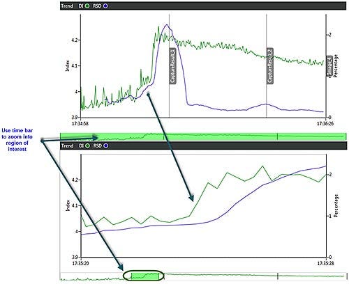
The Dispersion Index (DI) measures the entropy or disorder of the intensity in each frame and is displayed as a real-time trend plot. It monitors changes in the sample’s dispersion state. A higher DI value indicates a “busier” frame.
|
The Relative Standard Deviation (RSD) is calculated over a series of frames. It is a measure of the rate of change or variation of the DI over time.
|
|
|
Note: The Dispersion Index parameters can be used in conjunction with the laser obscuration and in particular the Dv90 values measured by the Mastersizer to identify the sample processes occurring during measurements.
| Recommended PC specification | Operating system : Windows 7 Ultimate (32 bit and 64 bit), Windows 8 Enterprise (64bit) Hardware specification: Intel Core i7 processor, 4GB RAM, 250GB HD, Wide screen monitor. |
| Set up. | Install the Hydro Sight Demo software and copy the three pre-recorded sample dispersion videos to ‘Sample Videos’ located in C:\Users\Public\Public Videos\Sample Videos |
| Launch the Hydro Sight SW by clicking on the desk top icon, if you selected to create one during install, or via the start menu. |
 C:\Program Files (x86)\Malvern Instruments\Hydro Sight (SELF DEMO)
 |
| Note: After showing the results for one pre-recorded sample dispersion video, it is necessary to close and restart the before running another video. | |
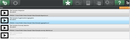
On starting the software you can choose which of the three example pre-recorded sample dispersion videos to measure.
Initially choose Example of Dispersion.
|
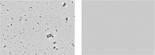
Initially a few frames of the sample will be observed in the video window – at this point the flat field correction is being performed and the sample name box will remain grayed out.
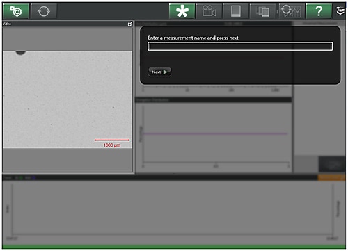
|
|
Note: A folder will be created with the path C:\Users\Public\Documents\Hydro Sight\[measurement name].
All images, videos (not available in the demo version) and saved results related to the measurement will be located here.
Note: In a real measurement you would now initialize the laser diffraction system and perform the background. Once the sample was introduced and the required obscuration level achieved you would be ready to start the Hydro Sight measurement.
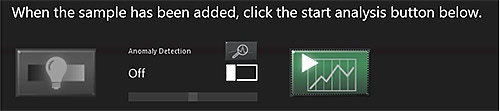
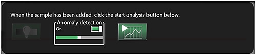
You will be prompted to select anomaly detection level. By default it is disabled (for now leave it off)
The sample ready button is also now active and you can press it (indicating the sample has been added and the laser diffraction system is ready for measurement).
|
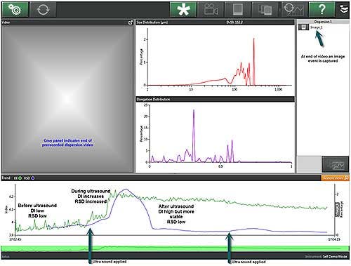
The rest of the pre-recorded video will now play in the live view window. Initially you may want to leave it to play all the way through and see the sample dispersing as described below.
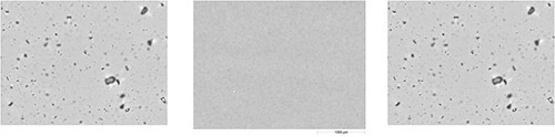
At the end of the video the live view will become blank and an image event will be captured. You will be able to see the full dispersion profile result in the lower part of the window. In the annotated screen shot below we have marked when ultrasound was applied and where the end of video event was indicated.
|
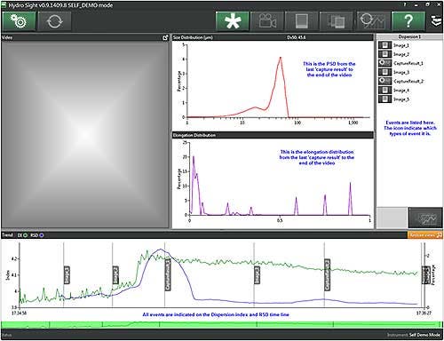
Run the same video again but this time capture measurements at different points during the disperison, such as where ultrasound was applied, using the capture event buttons at the top of the window. The various capture event buttons are described below.
Capture event options.
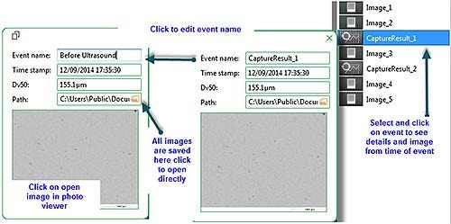
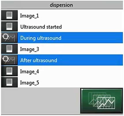
Each time an event button is pressed, the Size, Elongation and Dispersion Index graphs at that point in time will be captured in the event list along with an example image(s) of the dispersion at that time. In addition, the capture result button will also reset the graphs.
Image frame(s) and video are automatically saved in a sub folder called ‘Images’ within the folder created at the start of the measurement (eg C:\Users\Public\Documents\Hydro Sight\[measurement name]\Images).
NOTE: If any of the captured graphs are required for future use they will need to be saved via the review charts window.

|
Save a single image frame of the dispersion and capture the result at that point in time without resetting graphs.

|
Save a burst of image frames; the previous 10 frames which is approximately 2 seconds of data. For example to capture a feature you just observed that is no longer in view.

|
Capture result and reset graphs. As per save a single image frame, but this time the graphs will also be reset.

|
Capture video allows time limited videos of the dispersion to be recorded (30 sec, 1 min or 2 mins in duration). Video files are saved in the folder created at the start of the measurement and will be available to play back via windows media player.
Note: this is not available in the demo mode of the Software and is therefore greyed out. Here we see another measurement of the same pre-recorded dispersion shown earlier. This time events have been captured and the graphs reset during the dispersion process at approximately the times when ultrasound was applied.
|
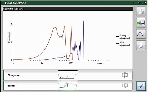
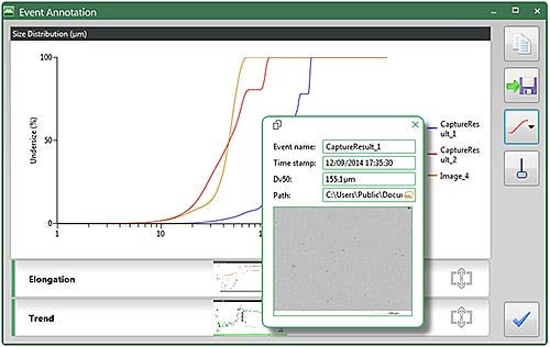
Captured results are temporarily saved in the events list from where they can be reviewed and annotated in the software. If a permanent record of the result is required it must be saved via the review charts button.
|
|
|
|
|
|

|

|

|
| Frequency
| Undersize
| Frequency and undersize
|
|
|
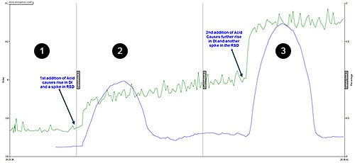
Here we can see the first application of ultrasound caused a relatively large step in the Dispersion Index and a large spike in the RSD. The second period of ultrasound caused a much smaller spike in the RSD and little change in the DI thus the sample was almost fully dispersed at this point.
Results can be saved as an image or copied to the clip board to paste in other applications

|
Results are saved as PNG images. Clicking the Export button saves out all three graphs and any annotation present.
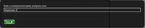
Save to the folder created at the start of the measurement (e.g. C:\Users\Public\Documents\Hydro Sight\Dispersion 1\Charts) or navigate as required.

|
Results can be copied to the clipboard to paste in other applications such as Microsoft Word or Power Point for reporting purposes
Note: After showing the results for one pre-recorded sample dispersion video, it is necessary to close and restart the software before running another video.
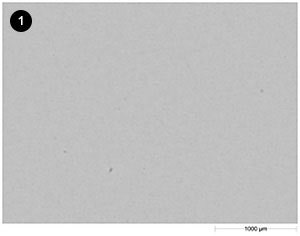
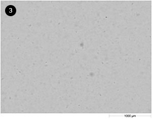
In this example milk is dispersed but has been caused to aggregate by the addition of acid. As with the previous dispersion example, the flat field correction is performed during the first few frames that are observed in the video window.
|
|

|
|
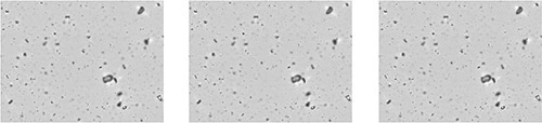
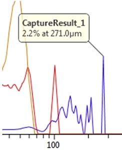
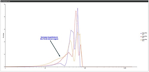
Capturing results where indicated saves example frames showing increasing numbers of observable particles. A small increase in the overall PSD is observed but more importantly the number of particles in the 10-30 µm region increases.
|
Anomalous frames may be automatically detected if the option is enabled at the start of a measurement.
|
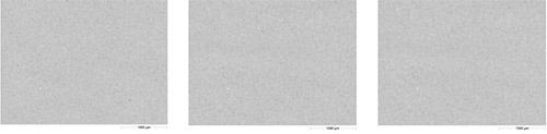
The anomaly detection is based on a measure of the standard deviation of pixel intensity (StDevPI) across a frame with respect to preceding frames. Frames with a StDevPI that falls outside the expected range, based on the previous frames, due to the presence of darker or brighter areas (particles) are automatically captured when the anomaly detection option is enabled. There are three levels of sensitivity available: low, medium and high.
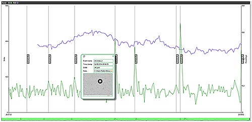
In the example of anomaly detection pre-recorded video, mono-modal latex beads are being measured which have been contaminated with a few large glass beads. Try using the different anomaly detection settings.
An anomaly event is automatically captured in the events list and the corresponding image is saved to the folder created at the start of the measurement. Clicking on the event either in the event list or on the DI chart reveals the image of the anomalous particle. This may be useful in trouble shooting applications for identifying the causes of an unexpected laser diffraction result. Anomaly detection can be enabled/disabled after starting measurement via the settings tab.
|
This technical note should help you become familiar with the Hydro Sight software. You can find more information about the Hydro Sight accessory from the Malvern website.

By clicking on this button from within the demo software you can ‘Request A Quote’ directly. This will take you back to the relevant page on the Malvern website.