Many industrial and biochemical applications depend on the usage of detergents and other surfactants. These compounds are indispensable, in particular, for the extraction, purification, and handling of membrane proteins. Owing to their amphiphilic nature, detergents can provide a membrane-mimetic environment required by integral membrane proteins to retain their native structures and functions in aqueous solution. Oftentimes, different detergents have to be screened to identify one that is suitable for the solubilization, stabilization, reconstitution, and biophysical, biochemical, or structural scrutiny of the protein of interest [1]. In each case, the membrane protein of interest dictates the suitability of a detergent, the choice of which depends on physicochemical properties such as chain length, headgroup size, and headgroup charge or polarity. However, a detergent found to be optimal for the isolation of a membrane protein need not necessarily be the best choice for downstream purification and in vitro studies. Harsh detergents such as SDS might inactivate the protein; some detergents such as Triton-X 100 absorb in the UV range and thus interfere with spectroscopic analysis; ionic detergents are unsuitable for isoelectric focusing or ion-exchange chromatography; and some detergents pose difficulties during membrane-protein reconstitution, that is, the reincorporation of the solubilized membrane protein into a lipid bilayer. Dialysis is a popular method for detergent removal to accomplish reconstitution, but long dialysis durations are required to remove detergents that have a low critical micellar concentration (CMC).
The CMC is one of the most fundamental characteristics of a surfactant. In aqueous solutions, surfactants form colloidal aggregates, so-called micelles, when their concentration exceeds the CMC. As abrupt changes of various physical properties are observable at or around this detergent concentration [2], its experimental determination can be realized with a variety of methods, including surface tension and conductivity measurements, dye binding experiments, and nuclear magnetic resonance spectroscopy [3]. To obtain the CMC in an accurate and precise manner, however, isothermal titration calorimetry (ITC) is the method of choice [4], which is due to its extraordinary sensitivity, unsurpassed resolution, and high reproducibility [5]. Moreover, ITC does not require sample labeling and provides a complete thermodynamic profile for a single experiment including the molar enthalpy and entropy changes accompanying micellization.
For these reasons, ITC has been used extensively for the determination of CMCs for a great variety of surfactants, including non-ionic surfactants such as alkylglucosides and -maltosides, alkyl phenol ethoxylates, oligo(ethylene oxide) alkylethers, and Tritons [ 6], zwitterionic surfactants such as 3 ([3 cholamidopropyl]dimethylammonio)-1 propanesulfonate CHAPS [ 6] and N,N dimethylaminedodecyl-n oxide [ 7], zwitterionic surface-active ionic liquids [ 8], anionic surfactants such as sodium dodecyl sulfate [ 9], sodium oleate, and bile salts [ 10], and cationic surfactants including such as alkylpyrinidinium halides [ 11], alkyltrimethylammonium bromides [ 12], and phosphonium gemini surfactants [ 13]. Moreover, ITC has been employed to determine the CMCs of fluorinated surfactants [ 14] and block copolymers [ 15, 16], surface-active peptides [ 17] and proteins [ 18], as well as of amino-acid-type surfactants [ 19] and amino-functionalized lipids [ 20].
To extract the CMC and the heat of demicellization of a surfactant by means of ITC, two strategies for data analysis are commonly used. Either the first derivative of the heat of demicellization with respect to surfactant concentration is calculated, or a generic sigmoidal fit is applied to the demicellization isotherm. In this whitepaper, we outline how both approaches can be combined to provide a data-analysis strategy of superior reproducibility and without user bias, as the only user input required is the calorimetric dataset itself. Interpretation of the latter is based on a simple pseudophase separation model described in the first section of this whitepaper. In the following sections, the approach is briefly explained and illustrated with two case studies, namely, CMC determination for a nonionic alkyl maltoside detergent and a zwitterionic derivative of cholic acid.
In a typical ITC experiment for CMC determination, an aqueous suspension of surfactant at a concentration well above the CMC is titrated into the same aqueous solvent (i.e., water or buffer). The isotherm of such a demicellization titration is characterized by three distinct ranges: at surfactant concentration below the CMC, micelles dissociate into monomers; when the surfactant concentration approaches the transition range around the CMC, the first micelles appear; finally, upon further addition of micellar surfactant, micelles are merely diluted at almost constant monomer concentration.
The process of demicellization measured in an ITC experiment is the reverse of micelle formation, which can be described by different thermodynamic models. Common models either assume that only two species, namely, detergent monomers and micelles, are found throughout the entire process, as is the case for the pseudophase separation model (Fig. 1A) [21] and the closed-association model (Fig. 1B) [22], or take into account populations of detergent assemblies of intermediate aggregation numbers, as is the case for the isodesmic model (Fig. 1C) [23] and the cooperative aggregation model (Fig. 1D) [24].
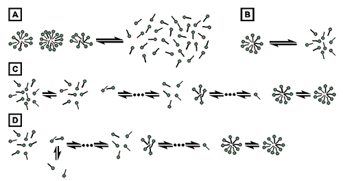
Fig. 1. Thermodynamic models of micelle formation. (A) Pseudophase separation model. (B) Closed-association model. (C) Isodesmic model. (D) Cooperative aggregation model.
The present analysis of demicellization isotherms is rooted in the pseudophase separation model, which considers monomers and micelles to be distinct pseudophases in equilibrium with each other (Fig. 1A) [21]. Note that this model makes no explicit assumptions as to the size or structure of micelles. By contrast, the closed-association model (also referred to as the “reversible two-state model” or “mass action model”, Fig. 1B) [22] does make particular assumptions about the size of the micelles and then regards micellization as a stoichiometric association reaction. For typical aggregation numbers >50, both of these models predict sudden changes in the physicochemical properties of the sample once the detergent concentration reaches the CMC. Contrastingly, the more gradual transitions usually observed experimentally are better reproduced by the isodesmic model or the cooperative aggregation model. The isodesmic model (Fig. 1C) [23] assumes stepwise aggregate formation, with each association step being characterized by the same association constant, whereas the cooperative aggregation model (Fig. 1D) [24] assumes dimer formation to be more difficult than all subsequent association steps. Although these two models are physically more realistic than the simpler models discussed above, they require additional fitting parameters and, therefore, are of limited practical value for the analysis of experimental micellization or demicellization data. Thus, in the absence of additional information warranting the use of these models, the pseudophase separation model is more robust and, hence, appears more suitable for the analysis of demicellization isotherms obtained from isothermal titration calorimetry.
For the majority of surfactants, a sigmoidal isotherm is obtained through integration of the demicellization thermogram. The transition range of such an isotherm is characterized by a relatively sharp decrease in the magnitude of the recorded heat. The isotherm yields the CMC as well as the heat of demicellization, Qdemic, by either of the two following approaches:
The local extremum (i.e., maximum or minimum, depending on the sign of the heat of demicellization) in the first derivative of the isotherm with respect to surfactant concentration within the transition range is taken as the CMC. Then, Qdemic is obtained from the difference in heat between linear pre- and post-transition baselines at the CMC [ 9].
A generic sigmoidal function is fitted to the isotherm to derive the CMC as well as Qdemic through nonlinear least-squares fitting [ 25, 14, 7].
The two approaches can be combined for a straightforward and unbiased analysis of demicellization isotherms, as described in detail in [ 26] and implemented into a Microsoft Excel worksheet. In brief, in a first step, the parameters describing the isotherm are estimated, including the CMC, the standard molar micellization enthalpy, 〖∆H°〗_mic, the slopes and ordinate intercepts of the pre-transition and post-transition baselines, m1, m2 and b1, b2, respectively, and ΔcD, which is a parameter describing the steepness of the isotherm. In a second step, these estimates are used as starting values for a nonlinear least-squares fit to the isotherm on the basis of a generic sigmoidal function according to the following equation:
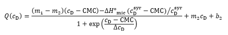
as described in detail elsewhere [ 26], with Q denoting the normalized heat of reaction and c_D the surfactant concentration in the calorimeter cell.
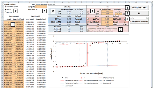
Fig. 2. Excel sheet provided for analysis of ITC demicellization isotherms. After isotherm data have been loaded and the total concentration of surfactant in the syringe has been provided by the user (1), estimate values of all fitting parameters are displayed immediately (2). After a nonlinear least-squares fit (3), fitting parameters are available (4) and can be assessed with regard to precision by means of confidence intervals (5). Additional checkboxes provide more options as specified in the text (0). Only values of orange cells should be modified.
Analysis of a demicellization isotherm with the Microsoft Excel worksheet involves the following steps (Figure 2):
Load your demicellization data in integrated and normalized form into the worksheet.
If peak integration was performed in Origin, export the table containing the integrated values as .dat file using default settings. If NITPIC [27] was used for baseline assignment and peak integration, just save the data as .dat. file. Then, in the spreadsheet, just click on the button “Load Data (.dat)”, choose the file of interest, and provide the total concentration of surfactant in the syringe.
If your data is in a format other than that provided by Origin or NITPIC, just paste your data into columns A (titrant concentration in mM) and B (integrated heats in cal/mol). Afterwards, provide the total concentration of surfactant in the syringe in cell D2.
After loading your data, the estimate values for parameters are calculated right away.
Check the estimates in the blue box and their graphical representation in the plot. At this point, if any of the estimates is not physically meaningful at all, enter your own estimate into the corresponding cell in the red box and uncheck the checkbox for the corresponding parameter to exclude it as a variable parameter from the fit to be performed in the next step.
Perform a nonlinear least-square fit to your data by clicking the “Fit” button. This procedure makes use of the Solver add-in bundled with Microsoft Excel as described in [ 28] and should only take some seconds to finish.
Check the resulting best-fit values in the red box and the fit in the plot. If a particular value looks suspicious or results in poor agreement of the fit with the experimental data, try changing and unchecking the corresponding parameter to keep it fixed and repeat the fit.
To assess the fitting precision of a best-fit value, choose the parameter of interest in the dropdown menu above the “Confidence Interval” button and click the latter. Wait until calculation of the confidence intervals is finished; this process may take some minutes. The sheet “Confidence Interval” is updated with the results of the confidence interval calculations. Repeat for confidence intervals of other parameters. If you want to keep the results for a parameter, click the “Keep CI Sheet” button on the “Confidence Interval” sheet.
In addition to this general procedure, the following options are available:
Toggle “Exclude first injection” to either include the data point corresponding to the first injection or exclude it. The latter option is set by default and recommended because the first injection usually suffers from syringe backlash and, possibly, sample loss during the mounting of the syringe and during sample equilibration and thus its corresponding heat is subject to large errors.
Toggle “Energy unit: kJ” to switch between kilojoules (kJ) and calories (kcal) (applies to all cells in the sheet and the plot). The input data, however, need to be given in cal/mol in any case.
Toggle “Use estimates as start values for variable parameters”. This option is enabled by default and should only be disabled if custom start values for the fitting procedure are desired. If disabled, custom start values entered into the corresponding cells of the red box are not overwritten by the estimates prior to the fitting procedure.
Toggle “Use estimates as values for fixed parameters”. If specific parameters are excluded as variable parameters from the fit, this option sets their estimates as fixed values. This option should be disabled if a parameter is to be set fixed at a custom value as in the case study below.
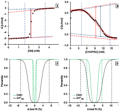
Fig. 3. Representative analysis of the demicellization of DM and CHAPSO as monitored by ITC. (A,B) Isotherms depicting integrated heats of reaction, Q, versus titrant concentration and (C,D) confidence interval for the adjustable parameters ΔH°mic and CMC are shown for the demicellization of (A,C) DM and (B,D) CHAPSO. (A,B) Experimental data (black solid circles), generic sigmoidal fit according to Eq. (1) (red open circles), pre-transition and post-transition baselines of initial estimate and fit (dotted and dashed blue and red lines, respectively), Qdemic at the CMC as derived from initial estimate and fit (blue and red solid lines, respectively), and estimated boundaries of transition region (vertical blue dashed lines). (C,D) Percentiles are plotted as functions of the relative deviations from best-fit values. Margins of 99% confidence intervals (dashed lines) are shown for the CMC (green) and ΔH°mic (black). These correspond to 2.21 mM and 2.26 mM with a best-fit value of 2.23 mM for the CMC of DM and to 8.91 mM and 9.75 mM with a best-fit value of 9.33 mM for that of CHAPSO. For the ΔH°mic of DM, they correspond to 4.68 kJ/mol and 5.35 kJ/mol with a best-fit value of 5.01 kJ/mol; for CHAPSO, they correspond to –3.51 kJ/mol and –2.98 kJ/mol with a best-fit value of –3.25 kJ/mol.
To exemplify the approach, demicellization experiments were carried out for the nonionic detergent n decyl-ß D maltoside (DM) [14] and the zwitterionic detergent 3 ([3 cholamidopropyl]dimethylammonio)-2 hydroxy-1 propanesulfonate (CHAPSO). Both titrations were performed on a VP-ITC instrument at a stirrer speed of 310 rpm and a filter period of 2 s. For DM demicellization, 24 mM detergent was titrated into triple-distilled water with a resistivity of 18 MΩ. The experiment was carried out at 25°C with a spacing of 300 s, a reference power of 63 µJ/s, and an injection volume of 10 µL (3 µL for first injection). For CHAPSO demicellization, 120 mM detergent was titrated into 20 mM sodium phosphate buffer at pH 7.0. The temperature was set to 35°C, the spacing to 750 s, the reference power to 13 µJ/s and the injection volume to 5 µL (3 µL for first injection). For data analysis, NITPIC [27] was used to assign baselines and to integrate thermogram peaks by singular value decomposition.
To obtain accurate and precise results from demicellization titrations, particular measures were taken during sample preparation, some of which apply to ITC experiments in general. Thus, buffers or water was filtered before use, and the exact same buffer was used for both samples in the syringe and the cell; otherwise, cosolute mixing might mask the heats arising from the process of interest (i.e., demicellization). For hygroscopic compounds in general and detergents in particular, it is important to allow them to equilibrate to room temperature before weighing them on a high-precision microbalance to avoid inaccuracies in stock concentrations. Furthermore, whereas degassing of samples is recommended for ITC measurements in general, it is advisable to refrain from degassing surfactant dispersions to prevent excessive foaming. To remove foam, samples can be centrifuged shortly at low speeds. As long as sufficient quantities of detergent are available, use of an ITC instrument with a large cell volume such as the VP-ITC is recommended to provide a higher signal-to-noise ratio.
Analysis of DM demicellization (Figure 3A) yielded initial estimates that were already close to the final best-fit values, as the experimental data comprised a sufficient number of injections (typically, at least 20) and displayed a good signal/noise ratio. This also resulted in narrow confidence intervals for all fit parameters of interest (Figure 3C).
By contrast, demicellization of CHAPSO gave rise to a more intricate isotherm, the pre-transition range of which exhibits a peak rather than a linear baseline. Owing to the steep rise of initial heats, the slope of the pre-transition baseline, m1, is overestimated, so that the fit yields physically unreasonable parameter values. However, this issue becomes obvious at a glance by comparison of the estimates with the best-fit values and by visual inspection of the graph and can be remedied by fixing m1 and m2 to zero and repeating the fit. In the absence of an educated guess on suitable values, use of the estimates is usually reasonable and can be effected by checking the option “Use estimates as values for fixed parameters”. The result of this approach is shown in Figure 3B. Although the confidence intervals are broader and slightly asymmetric for the DM dataset, they are still reasonably narrow (Figure 3D). Thus, even in such more complicated cases, only minimal user intervention is necessary to allow for a robust analysis of ITC demicellization data, and the solution can easily be identified. If further scrutiny is required, fixed values other than the estimates can be tried by unchecking the option “Use estimates as values for fixed parameters“. If, for example, both baseline slopes are fixed to zero for the CHAPSO data set, slightly narrower (i.e., by about 0.5% of the best-fit values) confidence intervals are obtained.
A possible reason for the difficulties encountered in the analysis of the CHAPSO isotherm lies in the fact that the micellization of this bile salt derivative results in micelles with a very small aggregation number (<10) and thus might be better explained by the closed-association model rather than by the pseudophase-separation model. Notwithstanding these uncertainties in the choice of fitting model, the best-fit value for the CMC of 9.33 mM is within the range of reported CMC values around 8 mM [ 29]. The slightly higher CMC as compared with this literature value can be attributed to the higher experimental temperature (CMC = 9.33 mM at 35°C as compared with 8 mM at 20°C), as the CMC is expected to increase with temperature because the micellization enthalpy is exothermic.
The two-step approach outline above provides both the CMC and ΔH°mic in an instant without requiring any additional user input other than the integrated and normalized isotherm and the surfactant concentration in the syringe. The demicellization analysis was implemented as a Microsoft Excel spreadsheet which is available from the authors and additionally allows for evaluation of the fit in terms of confidence intervals, as described elsewhere [28]. Extraction of CMC and ΔH°mic from demicellization isotherms using this analysis strategy provides fast and reproducible results without any user bias.
This whitepaper was authored by Martin Textor and Professor Dr. Sandro Keller, Molecular Biophysics, University of Kaiserslautern, Germany. Calorimetric titrations were conducted by Erik Frotscher and Johannes Klingler, University of Kaiserslautern, Germany.
Excel macro for analysis of ITC demicellization isotherms can be requested by mail from Professor Dr. Sandro Keller sandro.keller@biologie.uni-kl.de
Privé, G. G. Methods 41 (4), 388–397 (2007).
Preston, W. C. J. Phys. Colloid. Chem. 52, 84–96 (1948).
Natalini, B. et al. J. Pharm. Biomed. Anal. 87, 62–81 (2014).
Olofsson, G. and Loh, W. J. Braz. Chem. Soc. 20 (4), 577–593 (2009).
Bouchemal, K. et al. J. Mol. Recognit. 23 (4), 335–342 (2010).
Heerklotz, H. and Seelig, J. Biophys. J. 78 (5), 2435–2440 (2000).
Textor, M. et al. Methods 76, 183–193 (2015).
Wang, X. et al. J. Colloid Interface Sci. 391, 103–110 (2013).
Paula, S. et al. J. Phys. Chem. 99, 11742–11751 (1995).
Hildebrand, A. et al. Langmuir 20 (2), 320–328 (2004).
Bijma, K. and Engberts, J. B. F. N. Langmuir 10 (8), 2578–2582 (1994).
Beyer, K. et al. Colloids Surf. B. Biointerfaces 49 (1), 31–39 (2006).
Hemp, S. T. et al. Soft Matter 10 (22), 3970–3977 (2014).
Frotscher, E. et al. Angew. Chem. Int. Ed. 54 (17), 5069–5073 (2015).
Bouchemal, K. et al. J. Colloid Interface Sci. 338 (1), 169–176 (2009).
Rasolonjatovo, B. et al. Biomacromolecules 16 (3), 748–756 (2015).
Heerklotz, H. and Seelig, J. Biophys. J. 81 (3), 1547–1554 (2001).
Portnaya, I. et al. J. Agric. Food Chem. 54 (15), 5555–6155 (2006).
Ohta, A. et al. Colloids Surf. A Physicochem. Eng. Asp. 317 (1–3), 316–322 (2008).
Wölk, C. et al. Langmuir 30 (17), 4905–4915 (2014).
Shinoda, K. and Hutchinson, E. J. Phys. Chem 66 (4), 577–582 (1962).
Olesena, N. E. et al. Thermochimica Acta 588, 28-37 (2014).
Vickers, L. P. and Ackers, G. K. Arch. Biochem. Biophys. 174 (2), 747-749 (1976).
Beck, A. et al. J. Phys. Chem. B. 114 (48), 15862-15871 (2010).
Broecker, J. and Keller, S. Langmuir 29 (27), 8502–8510 (2013).
Textor, M. and Keller, S. Anal. Biochem., in press (2015).
Keller, S. et al. Anal. Chem. 84 (11), 5066–5073 (2012).
Kemmer, G. and Keller, S. Nat. Protoc. 5 (2), 267–281 (2010).
Kroflič, A. et al. Langmuir 28 (28), 10363-10371 (2012).