Basic Principles of Particle Size Analysis-1

Download



Basic Principles of Particle Size Analysis 

What is a particle?

  It would be a very foolish question to ask. However, with the various particle size analysis techniques, this becomes the foundation. The dispersion process and the shape of materials become more complex than in the initial particle size analysis.

Particle Size Issues

  Let’s assume someone gives you a matchbox and asks you to tell its size. You might say the matchbox size is 20*10*5mm. You can’t exactly answer the size as “20mm” because it’s one perspective of stating the size. Thus, you cannot describe a 3-dimensional matchbox with just one size. Clearly, this situation becomes more complex with particles of sand or pigment particles within a paint can. If I were a Q.A. (Quality Assurance) manager, I would want one number to describe particles – for example, to know if the average size of the latest batch of products is increasing or decreasing. This is a fundamental problem in the issue of particle size analysis – how can we represent a three-dimensional object with just one number?

Equivalent Spheres

  There is a sphere that can be expressed as a unique number. If we talk about a sphere with a size of 50μm, it can be accurately expressed. However, it is not possible to describe when referring to the edges and diagonals of a 50μm cube. A matchbox with many features can be expressed by one number. For example, the weight related to volume and surface area is one specific number. So, if there is a technique to measure the weight of the matchbox, we can convert the weight to that of a sphere. 

  Remember to calculate one specific number (2r) for the diameter of a sphere with the same weight as the matchbox. This is the equivalent sphere theory. We assume particles measured are spherical. Therefore, we obtain one specific number (the diameter of the sphere) to represent the particles.

   This tells you that when expressing a 3-dimensional particle, you don’t need to use three or more numbers, which may be inconvenient for control purposes but is more accurate.

   It can show interesting effects depending on the shape of the object, for example, demonstrating a cylinder like a sphere.

  However, if the shape or size of the cylinder changes, the volume/weight will differ. And as an equivalent spherical model, we can at least say it has gotten smaller or larger.

Equivalent Spherical Diameter of 100 x 20μm Cylinder

  Consider a cylinder with a diameter of D1=20μm and a height of 100μm. There is a sphere with a diameter of D2 which has the same volume as the cylinder. We can calculate the diameter as follows.

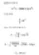
  The spherical diameter of a cylinder with a height of 100μm and a diameter of 20μm is approximately 40μm. The table below shows the equivalent spherical diameter of the cylinders at different ratios. The last row would be typical of a large clay particle in a disk shape, which tends to have a height of 20μm and a thickness of 0.2μm, generally not considering dimensions. Regarding devices that measure the volume of particles, you might get an answer around 5μm. Therefore, you need to use a different method to contest this result.

  Also, all these cylinders can appear in the same size as a filter with a 25μm, where you can say “everything is smaller than 25μm.” These cylinders may display different values during laser diffraction as they have different individual properties.

Various Measuring Techniques

  Obviously, if we see a particle under a microscope, we can see it projected in a 2-dimensional form and there are certain diameters of the particle that can be characterized and measured. If we accept the longest measurement of the particle and use it as our size, we may call the particle having a maximum dimension as a spherical particle. Similarly, if we use measurements like the minimum diameter or Feter’s diameter, this will provide us another answer regarding the particle’s size. We need to understand that each technique may measure different properties of a particle (maximum length, minimum length, volume, surface area, etc.). Therefore, if selectively measured, results will differ from other measurement techniques.

  Fig 3 shows several different answers that could describe a grain of sand. Each technique is not wrong – they all measure different characteristics of the particle. It’s like measuring the matchbox in cm or inches (you measure the length, and I’ll measure the width!).

  So, we can only compare measurements of powders obtained through the use of the same technique. This means that grains of sand do not have a standard size. The standard must be spherical through comparisons between each technique. However, we can obtain standard particle sizes with each technique, and this will lead to the comparison of equipment using these techniques.

D[4,3]etc

  Consider three spheres with dimensions of 1,2,3. What would the average size be among the three particles? Initially, we may say 2. How did we come to this answer? We sum all values and divide by the total number of particles.

 This is the number average (more accurately, the length average number). The number of particles can be expressed in equations.

  Mathematically, it’s called D[1,0]. The reason is that the diameter term in the equation above is represented by the quantity of (d1) while the bottom of the equation lacks a diameter term (d0). However, if I am an engineer related to catalysts, I would want to compare these spheres based on surface area. Because a higher surface area correlates to higher catalytic reactivity. The formula for the sphere’s surface area is 4πr2. Therefore, we must first find the square of the diameters divided by the number of particles and then take the square root for the average diameter.

  Again, this is a numerical average (average of the surface number). The reason is that the number of particles is represented in the below equation. We add up all the squares of the diameters. Thus, it is called mathematically as D[2,0]. – The upper term in the formula is squared and the diameter term is on the bottom. If I were a chemistry major, I would want to compare spheres based on fundamental weight. The formula for the weight of a sphere is as follows.

  Then, calculate the cubic root for the dimension that has divided by the number of particles to return to the average diameter.

  Once more, the average is found by dividing the number (number-volume or number-weight average). The reason the number of particles is reflected in the equation. In mathematical terms, this can be represented as D[3,0].

  The problem of simple averages of D[1,0], D[2,0], D[3,0] is inherent because of the unique nature of particle counting related to the formula. It requires counting large numbers of particles, which only takes place generally when it is a low count (ppm or ppb) for applications like contamination, control, and cleanliness. A simple calculation shows that if all particles of 1g of silica (density 2.5) were 1μm, then there would be approximately 760*10^9 particles.

Therefore, the concept of instantaneous averages needs to be supplemented, which could cause confusion. Two important averages are as follows.

• D[3,2]- Surface Area Average – Sauter Mean Diameter
• D[4,3]- Volume or Mass Average – De Brouckere Mean Diameter

  These averages are similar to moments of inertia, introducing another linear term associated with a different diameter (as shown below, surface area correlates with d3 and volume and mass correlate with d4).

  These formulas reflect the shift in the central point of frequency (surface area or volume/mass) distribution. In reality, they are the center of mass for each distribution. The advantage of this calculation method is evident – since the formula does not include the number of particles, the calculation and distribution of averages do not require knowledge of the number of complex particles. Laser diffraction initially calculates contributions based on volume terms. This is why D[4,3] is prominently reported.

Different Measurement Techniques Give Different Results

  If we use a grid-line-equipped electron microscope to measure particles to find out the diameter, then summarize or divide by the number of particles to get the average result. We count particles to find the average…” [Text truncated here due to input length.]